6.6 Random coin tosses
In this activity, we see an example of a sampling distribution that can be described by a normal distribution.
Use this website at RANDOM.org (at the bottom of the page, keep pressing Flip again to repeat) to flip ten Australian one-dollar coins at random (see Fig. 6.2).
Repeat this process numerous times (if you are in a class, each student can repeat the process numerous times so you get a large number of tosses), and complete the following table:
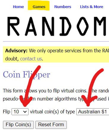
FIGURE 6.2: Using the online random coin-tosser.
| Proportion of heads in 10 tosses | How many times observed |
|---|---|
| 0.0 (0 heads) | |
| 0.1 (1 head) | |
| 0.2 (2 heads) | |
| 0.3 (3 heads) | |
| 0.4 (4 heads) | |
| 0.5 (5 heads) | |
| 0.6 (6 heads) | |
| 0.7 (7 heads) | |
| 0.8 (8 heads) | |
| 0.9 (9 heads) | |
| 1.0 (10 heads) | |
- Use this data to create a histogram of the proportion of heads. How would you describe the histogram?
- I also 'tossed' \(10\) coins, but repeated this random process \(400\) times. My histogram is shown in Fig. 6.3. How would you describe the histogram?
- Sketch the theoretical sampling distribution of the sampling proportion. What does this sketch show you?
- How would this sampling distribution change if we looked the proportion of heads in \(50\) tosses of a coin (rather than \(10\) tosses)?
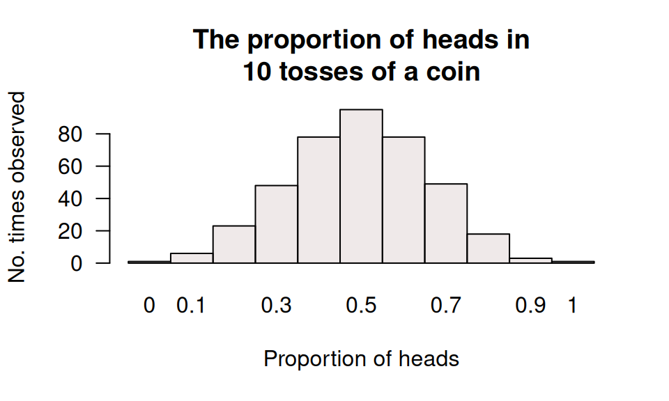
FIGURE 6.3: The histogram of the proportion of heads in \(10\) tosses, for \(400\) repetitions.