5 Mathematical expectation
Upon completion of this chapter, you should be able to:
- understand the concept and definition of mathematical expectation.
- compute the expectations of a random variable, functions of a random variable and linear functions of a random variable.
- compute the variance and other higher moments of a random variable.
- derive the moment generating function of a random variable and linear functions of a random variable.
- find the moments of a random variable from the moment generating function.
- state and use Tchebysheff’s inequality.
5.1 Expected values
Because random variables are random, knowing the outcome on any one realisation of the random process is not possible. Instead, we can talk about what might be expected to happen, or what might happen on average.
This is the idea of mathematical expectation. In more usual terms, the mathematical expression of a random variable is the mean. Mathematical expectation goes far beyond just computing means, but we begin here as the idea of a mean is easily understood.
The definition looks different in detail for discrete, continuous and mixed random variables, but the intention is the same.
Definition 5.1 (Expectation) The expectation or expected value (or mean) of a random variable \(X\) is written \(\operatorname{E}[X]\) (or \(\mu\), or \(\mu_X\) to distinguish between random variables).
For a discrete random variable \(X\) with PMF \(p_X(x)\), the expected value is \[ \operatorname{E}[X] = \sum_{x\in \mathcal{R}_X} x\cdot p_X(x). \] For a continuous random variable \(X\) with PDF \(f_X(x)\), the expected value is \[ \operatorname{E}[X] = \int_{-\infty}^\infty x\cdot f_X(x)\, dx. \]
For a mixed random variable \(X\), the expected value is \[ \operatorname{E}[X] = \sum_{x_i\in D} x_i \cdot p_X(X = x_i) + \int_S x \cdot f_X(x) \, dx, \] where \(D\) is the set of discrete mass points (with probability mass function \(p_X(x)\)) and \(S\) is the set of continuous intervals (with probability density function \(f_X(x)\)).
\(\operatorname{E}[X]\) is well-defined only if \(\operatorname{E}[\,|X|\,] < \infty\). If \(\int |x|f(x)\,dx = \infty\), the expectation does not exist (Example 5.28).
Effectively \(\operatorname{E}[X]\) is a weighted average of the points in \(\mathcal{R}_X\), the weights being the probabilities for each value of \(x\in \mathcal{R}_X\) in the discrete case and probability densities in the continuous case.
Example 5.1 (Expectation for discrete variables) Consider the discrete random variable \(U\) with probability function \[ p_U(u) = (u^2 + 1)/5 \qquad \text{(for $u = -1, 0, 1$)}, \] so that \(\mathcal{R}_U = \{-1, 0, 1\}\). The expected value of \(U\) is \[\begin{align*} \operatorname{E}[U] &= \sum_{\mathcal{R}_U} u\cdot p_U(u) \\ &= \sum_{\mathcal{R}_U} u \times\left( \frac{u^2 + 1}{5} \right) \\ &= \left( -1 \times \frac{(-1)^2 + 1}{5} \right ) + \left( 0 \times \frac{(0)^2 + 1}{5} \right ) + \left( 1 \times \frac{(1)^2 + 1}{5} \right ) \\ &= -2/5 + 0 + 2/5 = 0. \end{align*}\] The expected value of \(U\) is \(\operatorname{E}[U] = 0\).
Example 5.2 (Expectation for continuous variables) Consider a continuous random variable \(X\) with PDF \[ f_X(x) = x/4 \qquad \text{(for $1 < x < 3$)}. \] The expected value of \(X\) is \[\begin{align*} \operatorname{E}[X] &= \int_{-\infty}^\infty x\cdot f_X(x) \, dx = \int_1^3 x(x/4)\, dx\\ &= \left.\frac{1}{12} x^3\right|_1^3 = 13/6. \end{align*}\] The expected value of \(X\) is \(\operatorname{E}[X] = 13/6\).
Example 5.3 (Expectation for mixed variables) Consider a mixed random variable \(W\) with probability function \[ f_W(w) = \begin{cases} 1/2 & \text{for $w = 0$};\\ \exp(-2w) & \text{for $w > 0$} \end{cases} \] so that \(p_W(w) = 1/2\) for \(w = 0\), and \(f_W(w) = \exp(-2w)\) for \(w > 0\). The expected value of \(W\) is \[\begin{align*} \operatorname{E}[W] &= \overbrace{\sum_{w = 0} w\cdot p_W(w)}^{\text{Discrete component}} \quad + \quad \overbrace{\int_{-\infty}^\infty w\cdot f_W(w)\, dw}^{\text{Continuous component}}\\ &= \sum_{w = 0} 0\times (1/2)\quad + \quad \int_{0}^\infty w\times \exp(-2w)\, dw\\ &= 0 \quad + \quad 1/4\\ &= 1/4. \end{align*}\] The expected value of \(W\) is \(\operatorname{E}[W] = 1/4\).
Example 5.4 (Expectation for a coin toss) Consider tossing a coin once and counting the number of tails. Let this random variable be \(T\). The probability function is \[ p_T(t) = 0.5 \qquad \text{(for $t = 0, 1$)}. \] The expected value of \(T\) is \[\begin{align*} \operatorname{E}[T] &= \sum_{t = 1}^2 t\cdot p_T(t)\\ &= \Pr(T = 0) \times 0 \quad + \quad \Pr(T = 1) \times 1\\ &= (0.5 \times 0) + (0.5 \times 1) = 0.5. \end{align*}\] Of course, \(0.5\) tails can never actually be observed in practice on one toss. But it would be silly to round up (or down) and say that the expected number of tails on one toss of a coin is one (or zero). The expected value of \(0.5\) simply means that over a large number of repetitions of this random process, a tail is expected to occur in half of those repetitions.
Example 5.5 (Mean undefined) Consider the distribution of \(Z\), with the probability density function \[ f_Z(z) = z^{-2} \qquad \text{(for $z \ge 1$)} \] as in Fig. 5.1. The expected value of \(Z\) is \[ \operatorname{E}[Z] = \int_1^{\infty} z \frac{1}{z^2}\, dz = \int_1^\infty \frac{1}{z} = \left[\log z \right]_1^\infty. \] However, \(\displaystyle\lim_{z\to\infty}\, \log z \to \infty\). The expected value of \(\operatorname{E}[Z]\) is undefined.

FIGURE 5.1: The probability function for the random variable \(Z\). The mean is not defined.
Show R code
# Define values of z > 1 to plot over
z <- seq(1, 6, length.out = 100)

# Plot for z > 1
plot(x = z, y = z^(-2),
     type = "l", lwd = 2, las = 1,
     xlim = c(0, 6), ylim = c(-0.025, 1),
     xlab = "z", ylab = "Density",
     main = "Probability function for Z")

# Line for x = 0 to x = 1
lines( x = c(-1, 1), y = c(0, 0),
       lwd = 2) ### lwd = 2: Thicker line width

# Dotted vertical line
abline(v = 1, lty = 2, ### lty = 2: means 'dotted lines'
       col = "grey")

# Show open point
points(x = 1, y = 0,
       pch = 1) ### pch = 1: open circle
5.2 Expectation of a function of a random variable
The concept of mathematical expectation applies more widely than just to a random variable \(X\), using the following theorem.
Theorem 5.1 (Expectation for a function of a random variable) The expected value of some function \(g(\cdot)\) of a random variable \(X\) is written \(\operatorname{E}[ g(X)]\).
For a discrete random variable \(X\) with probability mass function \(p_X(x)\), the expected value of \(g(X)\) is \[ \operatorname{E}\big[g(X)\big] = \sum_{x\in \mathcal{R}_X} g(x)\cdot p_X(x). \] For a continuous random variable \(X\) with probability density function \(f_X(x)\), the expected value of \(g(X)\) is \[ \operatorname{E}\big[g(X)\big] = \int_{-\infty}^\infty g(x)\cdot f_X(x)\,dx. \] For a mixed random variable \(X\) with probability mass function \(p_X(x)\) and probability density function \(f_X(x)\), the expected value of \(g(X)\) is \[ \operatorname{E}\big[g(X)\big] = \sum_{x\in \mathcal{R}_X} g(x)\, p_X(x) + \int_{-\infty}^{\infty} g(x)\, f_X(x)\,dx, \] where \(\mathcal{R}_X\) is the set of values having positive probability mass.
Proof. The proof must be delayed until later (Example 9.13).
Example 5.6 (Expectation for a function of a discrete variable) Consider the discrete random variable \(U\) with probability function shown in Example 5.1: \[ p_U(u) = (u^2 + 1)/5 \qquad \text{for $u = -1, 0, 1$}. \] Define \(V = U^2\), where \(g(U) = U^2\). Since \(\mathcal{R}_U = \{-1, 0, 1\}\), then \(\mathcal{R}_V = \{ (-1)^2, 0^2, 1^2\} = \{0, 1\}\). Then the expected value of \(V\) is \[\begin{align*} \operatorname{E}[V] = \operatorname{E}[g(U)] &= \sum_{\mathcal{R}_U} g(u)\cdot p_U(u) \\ &= \left( (-1)^2 \times \frac{(-1)^2 + 1}{5} \right ) + \left( 0^2 \times \frac{(0)^2 + 1}{5} \right ) + \left( 1^2 \times \frac{(1)^2 + 1}{5} \right ) \\ &= 2/5 + 0 + 2/5 = 4/5. \end{align*}\] The expected value of \(V = U^2\) is \(\operatorname{E}[V] = 4/5\).
Example 5.7 (Expectation for a function of a continuous variable) Consider the continuous random variable \(X\) with probability density function shown in Example 5.2: \[ f_X(x) = x/4 \qquad \text{for $1 < x < 3$}. \] The expected value of \(Y = \sqrt{X}\), where \(g(X) = \sqrt{X}\), is \[\begin{align*} \operatorname{E}[Y] = \operatorname{E}[ g(X) ] &= \int_{-\infty}^\infty g(x)\cdot f_X(x) \, dx\\ &= \int_1^3 \sqrt{x}\times \frac{x}{4}\, dx\\ &= \frac{9\sqrt{3} - 1}{10}\approx 1.458... \end{align*}\] The expected value of \(Y = \sqrt{X}\) is \(\operatorname{E}[Y] = (9\sqrt{3} - 1)/10\).
Example 5.8 (Expectation for a function of a mixed variable) Consider the mixed random variable \(W\) with probability density function shown in Example 5.3. The expected value of \(Z = 1 - W\) is \[\begin{align*} \operatorname{E}[Z] &= \sum_{w=0} (1 - w)\cdot p_W(w) \quad + \quad \int_{0}^\infty (1 - w)\cdot f_W(w) \, dw\\ &= (1 - 0) \times\frac{1}{2} \quad + \quad \left[ \frac{1}{4}\exp(-2w) (2w - 1)\right]_0^\infty\\ &= \frac{1}{2} + (0 + \frac{1}{4}) = \frac{3}{4}. \end{align*}\] The expected value of \(Z = 1 - W\) is \(3/4\).
Importantly, the expectation operator is a linear operator.
Theorem 5.2 (Expectation properties) For any random variable \(X\) and constants \(a\) and \(b\), \[ \operatorname{E}[aX + b] = a\operatorname{E}[X] + b. \]
Proof. Assume \(X\) is a discrete random variable with probability function \(p_X(x)\). By Theorem 5.1 with \(g(X) = aX + b\), \[ \operatorname{E}[aX + b] = \sum_x (ax + b)\, p_X(x) = a\sum_x x\cdot p_X(x) + b\sum_x p_X(x) = a\operatorname{E}[X] + b, \] using that \(\sum_x p_X(x) = 1\). (The proof in the continuous case is similar, but the probability function is a PDF and integrals replace summations.)
Example 5.9 (Expectation of a function of a random variable) Consider the random variable \(Z = 2X\) where \(X\) is defined in Example 5.2. Using Theorem 5.2 with \(a = 2\) and \(b = 0\), the value of \(\operatorname{E}[Z]\) is \[ \operatorname{E}[Z] = \operatorname{E}[2X] = 2\operatorname{E}[X] = 2 \times 13/6 = 13/3. \]
Example 5.10 (Expectation for a function of a mixed variable) Consider the mixed random variable \(W\) with probability density function shown in Example 5.3. The expected value of \(Z = 1 - W\), which is a linear transformation, was shown in Example 5.8 to be \(3/4\). Since \(Z\) is a linear transformation, we could also proceed: \[ \operatorname{E}[Z] = \operatorname{E}[1 - W] = 1 - \operatorname{E}[W] = 1 - \frac{1}{4} = \frac{3}{4} \] using \(\operatorname{E}[W] = 1/2\) from Example 5.3. The answer is, of course, the same answer found in Example 5.8.
An important result that follows is Jensen’s inequality, which applies for convex and concave functions which we first define.
Definition 5.2 (Convex and concave functions) A twice-differentiable function \(g(\cdot)\) is convex on an interval \(I\) if \[ g''(x) \geq 0 \quad \text{for all } x \in I, \] and strictly convex if \(g''(x) > 0\) for all \(x \in I\).
The function \(g(\cdot)\) is concave on an interval \(I\) if \[ g''(x) \leq 0 \quad \text{for all } x \in I, \] and strictly concave if \(g''(x) < 0\) for all \(x \in I\).
Example 5.11 (Concave and convex functions) The function \(g(x) = x^2\) is strictly convex over \(\mathbb{R}\) (Fig. 5.2, left panel), because \[ g''(x) = 2 > 0 \] for all real values of \(x\). Similarly, the function \(g(x) = \log x\) is strictly concave over the interval \(I = (0, \infty)\) (Fig. 5.2, right panel), because \[ g''(x) = -\frac{1}{x^2} < 0 \] for all values of \(x\in I\).
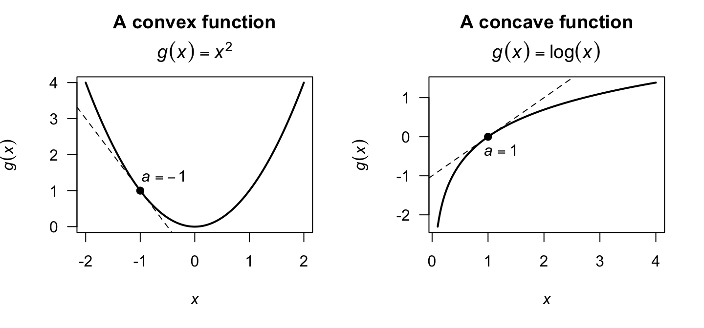
FIGURE 5.2: A convex function (left) and a concave function (right). The dashed lines are the tangents at a fixed point \(x = a\).
One important observation for a convex function is that the tangent line at any point \(a\) is a global underestimate of the function; that is, \(g(x) \geq g(a) + g'(a)(x - a)\) for all \(x \in I\). Contrast the tangents in the left and right panels of Fig. 5.2.
Theorem 5.3 (Jensen's inequality) Let \(X\) be a random variable and \(g(\cdot)\) a convex function. Then \[ g(\operatorname{E}[X]) \leq \operatorname{E}[g(X)]. \] If \(g(\cdot)\) is strictly convex, equality holds if and only if \(X\) is degenerate; that is, \(\Pr(X = c) = 1\) for some constant \(c\).
Similarly, if \(g(\cdot)\) is a concave function, then \[ g(\operatorname{E}[X]) \geq \operatorname{E}[g(X)]. \]
Proof. We prove the case for convex function only. Since \(g(\cdot)\) is convex, the value of \(g(x)\) lies above every tangent line (see Fig. 5.2, left panel) at every point \(x_0\in I\). Assume the tangent line at \(x = x_0\) has a slope \(b\); then this implies that \[ g(x) > g(x_0) + b(x - x_0). \] If we set \(x_0 = \mu = \operatorname{E}[X]\), then \[ g(x) > g(\mu) + g'(\mu)(x - \mu) \quad \text{for all } x. \] Taking expectations of both sides, \[\begin{align*} \operatorname{E}[g(X)] &> g(\mu) + g'(\mu)\operatorname{E}[X - \mu]\\ &= g(\mu) + g'(\mu) \times 0\\ &= g(\operatorname{E}[X]). \end{align*}\]
Common convex functions to which Jensen’s inequality applies include \(g(x) = x^2\), \(g(x) = \exp x\), \(g(x) = -\log x\) (\(x > 0\)), and \(g(x) = 1/x\) (\(x > 0\)).
For concave \(g(\cdot)\) the inequality reverses: \(\operatorname{E}[g(X)] \leq g(\operatorname{E}[X])\); a common example is \(g(x) = \log x\).
Example 5.12 (Jensen's inequality applied) Let \(X > 0\) be a non-degenerate random variable with \(\operatorname{E}[X] = \mu\). Since \(g(x) = 1/x\) is strictly convex for \(x > 0\), Jensen’s inequality gives \[ \operatorname{E}\!\left[\frac{1}{X}\right] > \frac{1}{\operatorname{E}[X]} = \frac{1}{\mu}. \]
5.3 The variance and standard deviation
Apart from the mean, the most important description of a random variable is the variability: quantifying how the values of the random variable are dispersed. The most important measure of variability is the variance.
The variance of a random variable is a measure of the variability of a random variable. (More correct is to say ‘the variance of the distribution of the random variable’ rather than ‘variance of a random variable’, but this language is commonly used.) A small variance means the observations are nearly the same (i.e., small variation); a large variance means they are quite different. The variance can be expressed as a function of a random variable.
Definition 5.3 (Variance) The variance of a random variable \(X\) (or, of the distribution of \(X\)) is \[ \operatorname{var}[X] = \operatorname{E}\big[(X - \mu)^2\big] \] where \(\mu = \operatorname{E}[X]\). The variance of \(X\) is commonly denoted by \(\sigma^2\), or \(\sigma^2_X\) if distinguishing among variables is needed.
The variance is the expected value of the squared distance of the values of the random variable from the mean, weighted by the probability function. The unit of measurement for variance is the original unit of measurement squared. That is, if \(X\) is measured in metres, the variance of \(X\) is in \(\text{metres}^2\).
Describing the variability in terms of the original units is more natural, by taking the square root of the variance.
Definition 5.4 (Standard deviation) The standard deviation of a random variable \(X\) is defined as the positive square root of the variance (denoted by \(\sigma\)); i.e., \[ \operatorname{sd}[X] = \sigma = +\sqrt{\operatorname{var}[X]} \]
The variance is less popular than the standard deviation in practice to describe variability. In theoretical work, however, the variance is easier to work with than standard deviation (due to the square root), and the variance, rather than standard deviation, features in many results in theoretical statistics.
Example 5.13 (Variance for a die toss) Suppose a fair die is tossed, and \(X\) denotes the number of points showing. Then \(\Pr(X = x) = 1/6\) for \(x = 1, 2, 3, 4, 5, 6\) and \[ \mu = \operatorname{E}[X] = \sum_S x\cdot p_X(x) = (1 + 2 + 3 + 4 + 5 + 6 )/6 = 7/2. \] The variance of \(X\) is then \[\begin{align*} \sigma^2 &= \operatorname{var}[X] = \sum (X - \mu)^2 p_X(x)\\ &= \frac{1}{6}\left[ \left(1 - \frac{7}{2}\right)^2 + \left(2 - \frac{7}{2}\right)^2 + \dots + \left(6 - \frac{7}{2}\right)^2 \right] = \frac{70}{24}. \end{align*}\] The standard deviation is then \(\sigma = \sqrt{70/24} \approx 1.71\).
An important result is the computational formula for variance, which is usually easier to use in practice than the formula given in Definition 5.3.
Theorem 5.4 (Computational formula for variance) For any random variable \(X\), \[ \operatorname{var}[X] = \operatorname{E}[X^2] - \operatorname{E}[X]^2. \]
Proof. Let \(\operatorname{E}[X] = \mu\), then (using the properties of expectation in Theorem 5.2): \[\begin{align*} \operatorname{var}[X] = \operatorname{E}\left[(X - \mu)^2\right] &= \operatorname{E}\left[X^2 - 2X\mu + \mu^2\right] \\ &= \operatorname{E}[X^2] - \operatorname{E}[2X\mu] + \operatorname{E}\left[\mu^2\right]\quad\text{(since $\operatorname{E}[\cdot]$ is a linear operator)}\\ &= \operatorname{E}[X^2] - 2\mu\operatorname{E}[X] + \mu^2\\ &= \operatorname{E}[X^2] - 2\mu^2 + \mu^2 \\ &= \operatorname{E}[X^2] - \mu^2 \\ &= \operatorname{E}[X^2] - \operatorname{E}[X]^2. \end{align*}\]
This formula is often easier to use to compute \(\operatorname{var}[X]\) than using the definition directly.
Example 5.14 (Variance for a die toss) Consider Example 5.13 again. Then \[\begin{align*} \operatorname{E}[X^2] = \sum_S x^2 \cdot p_X(x) &= \frac{1}{6}(1^2 + 2^2 + 3^2 + 4^2 + 5^2 + 6^2)\\ &= 91/6, \end{align*}\] and so \(\operatorname{var}[X] = 91/6 - (7/2)^2 = 70/24\), as before.
Example 5.15 (Variance using computational formula) Consider the continuous random variable \(X\) with PDF \[ f_X(x) = 3x(2 - x)/4 \qquad \text{for $0 < x < 2$}. \] The variance of \(X\) can be computed in two ways: using \(\operatorname{var}[X] = \operatorname{E}[(X - \mu)^2]\) or using the computational formula. The expected value of \(X\) is \[ \operatorname{E}[X] = \int_0^2 x\times 3x(2 - x)/4\, dx = 1. \] To use the computational formula, also find \[ \operatorname{E}[X^2] = \frac{6}{5}, \] and so \(\operatorname{var}[X] = \operatorname{E}[X^2] - \operatorname{E}[X]^2 = 1/5\).
Using the definition, \[\begin{align*} \operatorname{var}[X] = \operatorname{E}\big[(X - \operatorname{E}[X])^2\big] &= \operatorname{E}\big[(X - 1)^2\big]\\ &= \int_0^2 (x - 1)^2 \times 3x(2 - x)/4\,dx = 1/5. \end{align*}\] Both methods give the same answer, and both methods require initial computation of \(\operatorname{E}[X]\).
Example 5.16 (Variance for a mixed variable) Consider the mixed random variable \(W\) with probability density function shown in Example 5.3. The expected value of \(W\) is \(\operatorname{E}[W] = 1/4\). The variance of \(W\) is then \(\operatorname{var}[W] = \operatorname{E}[W^2] - \operatorname{E}[W]^2\), and so \[\begin{align*} \operatorname{E}[W^2] &= \overbrace{\sum_{w = 0} w^2\,p_W(w)}^{\text{Discrete component}} \quad + \quad \overbrace{\int_{-\infty}^\infty w^2\, f_W(w)\,dw}^{\text{Continuous component}}\\ &= 0^2\times \frac12 \quad + \quad \int_0^\infty w^2 e^{-2w}\,dw\\ &= \frac{1}{4}. \end{align*}\] Therefore \[ \operatorname{var}[W] = \frac{1}{4}-\frac{1}{16} = \frac{3}{16}. \]
The variance represents the expected value of the squared distance of the values of the random variable from the mean. The variance is never negative, and is only zero when all the values of the random variable are identical (that is, there is no variation in the values of \(X\)).
If most of the probability lies near the mean, the dispersion will be small; if the probability is spread out over a considerable range the dispersion will be large.
Example 5.17 (Variance undefined) In Example 5.5, \(\operatorname{E}[X]\) was not defined. For that reason, the variance is also undefined, since computing the variance relies on having a finite value for \(\operatorname{E}[X]\).
Theorem 5.5 (Variance properties) For any random variable \(X\) and constants \(a\) and \(b\), \[ \operatorname{var}[aX + b] = a^2\operatorname{var}[X]. \]
Proof. Using the computational formula for the variance: \[\begin{align*} \operatorname{var}[aX + b] &= \operatorname{E}\left[ (aX + b)^2 \right] - \left(\operatorname{E}[aX + b] \right)^2\\ &= \operatorname{E}\left[a^2 X^2 + 2abX + b^2\right] - (a\mu+b)^2\\ &= a^2 \operatorname{E}[X^2] - a^2\mu^2\\ &= a^2 \operatorname{var}[X]. \end{align*}\]
The special case \(a = 0\) is instructive: \(\operatorname{var}[b] = 0\) when \(b\) is constant. In other words, a constant has zero variation, as expected.
Example 5.18 (Variance of a function of a random variable) Consider the random variable \(Y = 4 - 2X\) where \(\operatorname{E}[X] = 1\) and \(\operatorname{var}[X] = 3\). Then: \[\begin{align*} \operatorname{E}[Y] &= \operatorname{E}[4 - 2X] = 4 - 2\times\operatorname{E}[X] = 2;\\ \operatorname{var}[Y] &= \operatorname{var}[4 - 2X] = (-2)^2\operatorname{var}[X] = 12. \end{align*}\]
5.4 Tchebysheff’s inequality
Tchebysheff’s inequality applies to any probability distribution, and is sometimes useful in theoretical work or to provide bounds on probabilities.
Theorem 5.6 (Tchebysheff's theorem) Let \(X\) be a random variable with finite mean \(\mu\) and variance \(\sigma^2\). Then for any positive \(k\), \[\begin{equation} \Pr\big(|X - \mu| \geq k\sigma \big)\leq \frac{1}{k^2} \tag{5.1} \end{equation}\] or, equivalently \[\begin{equation} \Pr\big(|X - \mu| < k\sigma \big)\geq 1 - \frac{1}{k^2}. \end{equation}\]
Proof. The proof for the continuous case only is given. Let \(X\) be continuous with PDF \(f(x)\). For some \(c > 0\), then \[\begin{align*} \sigma^2 & = \int^\infty_{-\infty} (x - \mu )^2 f(x)\,dx\\ & = \int^{\mu -\sqrt{c}}_{-\infty} (x - \mu )^2 f(x)\, dx + \int^{\mu + \sqrt{c}}_{\mu-\sqrt{c}}(x - \mu )^2 f(x)\,dx + \int^\infty_{\mu + \sqrt{c}}(x - \mu)^2 f(x)\,dx\\ & \geq \int^{\mu -\sqrt{c}}_{-\infty} (x - \mu )^2 f(x)\,dx + \int^\infty_{\mu + \sqrt{c}}(x - \mu )^2 f(x)\,dx, \end{align*}\] since the second integral is non-negative. Now \((x - \mu )^2 \geq c\) if \(x \leq \mu -\sqrt{c}\) or \(x\geq \mu + \sqrt{c}\). So in both the remaining integrals above, replace \((x - \mu )^2\) by \(c\) without altering the direction of the inequality: \[\begin{align*} \sigma^2 &\geq c \int^{\mu -\sqrt{c}}_{-\infty} f(x)\,dx + c\int^\infty_{\mu + \sqrt{c}}f(x)\,dx\\ &= c\,\Pr(X \leq \mu - \sqrt{c}\,) + c\,\Pr(X \geq \mu + \sqrt{c}\,)\\ &= c\,\Pr(|X - \mu| \geq \sqrt{c}\,). \end{align*}\] Putting \(\sqrt{c} = k\sigma\), Eq. (5.1) is obtained.
With the probability function or PDF of a random variable \(X\), then \(\operatorname{E}[X]\) and \(\operatorname{var}[X]\) can be found, but the converse is not true. That is, from a knowledge of \(\operatorname{E}[X]\) and \(\operatorname{var}[X]\) we cannot reconstruct the probability distribution of \(X\) and hence cannot compute probabilities such as \(\Pr(|X - \mu| \geq k\sigma)\). Nonetheless, using Tchebysheff’s inequality we can find a useful bound to either the probability outside or inside of \(\mu \pm k\sigma\).
Example 5.19 (Tchebysheff inequality) Suppose students’ exam marks \(X\) have mean \(70\) and standard deviation \(10\). Tchebysheff’s inequality can be used to bound the probability that a student’s mark differs from the mean by at least \(20\) marks.
Since \(|X - \mu| \ge 20\) and \[ k = 20/10 = 2, \] Tchebysheff’s inequality gives \[ \Pr( |X - \mu| \ge k\sigma) \le 1/k^2; \] hence \[ \Pr( |X - 70| \ge 20) \le 1/2^2 = 1/4. \] Therefore \[ \Pr(| X - 70 | \ge 20) \le 0.25, \] or, equivalently, \[ \Pr(50 < X < 90) \ge 0.75. \] Even if we know nothing about the distribution of marks, and only know the mean and standard deviation, we can still guarantee that at least \(75\)% of marks lie between \(50\) and \(90\).
5.5 Higher moments
5.5.1 Raw and central moments
The ideas of a mean and a variance can be generalised. The mean is a special case of a ‘raw moment’, and the variance is a special case of a ‘central moment’.
Definition 5.5 (Raw moments) The \(r\)th raw moment, or \(r\)th moment about the origin, of a random variable \(X\) (where \(r\) is a positive integer) is denoted \(\mu'_r\) and defined as \(\mu'_r = \operatorname{E}[X^r]\).
For a discrete random variable \(X\), the \(r\)th moment about the origin is \[ \mu'_r = \operatorname{E}[X^r] = \sum_X x^r\cdot p_X(x). \] For a continuous random variable \(X\), the \(r\)th moment about the origin is \[ \mu'_r = \operatorname{E}[X^r] = \int_{-\infty}^\infty x^r\cdot f_X(x)\, dx \]
Definition 5.6 (Central moments) The \(r\)th central moment, or \(r\)th moment about the mean (where \(r\) is a positive integer), is denoted \(\mu_r\) and defined as \(\mu_r = \operatorname{E}[(X - \mu)^r]\).
For a discrete random variable \(X\), the \(r\)th central moment is \[ \mu_r = \operatorname{E}[(X - \mu)^r] = \sum_x (x - \mu)^r\cdot p_X(x). \] For a continuous random variable \(X\), the \(r\)th central moment is \[ \mu_r = \operatorname{E}\big[(X - \mu)^r\big] = \int_{-\infty}^{\infty} (x - \mu)^r\cdot f_X(x)\, dx. \]
From these definitions:
- the mean \(\mu'_1 = \mu\) is the first raw moment;
- \(\mu'_2 = \operatorname{E}[X^2]\) is the second raw moment; and
- the variance \(\mu_2 = \sigma^2\) is the second central moment.
5.5.2 Skewness
Higher moments also exist that describe other features of a random variable beyond the mean and variance. The third central moment is related to skewness, a measure the asymmetry of a distribution.
Definition 5.7 (Symmetry) The distribution of \(X\) is said to be symmetric if, for all \(x\in \mathcal{R}_X\),
- \(p_X(\mu + x) = p_X(\mu - x)\) for a discrete random variable \(X\) with PMF \(p_X(x)\), or
- \(f_X(\mu + x) = f_X(\mu - x)\) for a continuous random variable \(X\) with PDF \(f_X(x)\),
where \(\mu = \operatorname{E}[X]\) is the mean of \(X\).
For a symmetric distribution, the odd central moments are zero (Exercise 5.19). This suggests that the odd central moments (such as the third central moment) can be used to measure the asymmetry of a distribution.
However, rather than using the third central moment explicitly, by applying Def. 5.6, finding the appropriate expected value of a normalised version of the random variable (i.e., with mean zero and variance one) is preferred. That is, the definition of skewness finds the appropriate expected value of \((X - \mu)/\sigma\) rather than of \(X\) directly. This means that the value of the skewness for the random variable \(X\) is unaffected by a linear transformation of the type \(Y = aX + b\) (for constants \(a\) and \(b\)).
Definition 5.8 (Skewness) The skewness of the distribution of a random variable \(X\) with mean \(\operatorname{E}[X] = \mu\) and variance \(\operatorname{var}[X] = \sigma^2\) is defined as \[\begin{align} \text{skewness} = \gamma_1 &= \operatorname{E}\left[\left(\frac{X-\mu}{\sigma}\right)^3\right]\notag\\ &= \frac{\mu_3}{(\sigma^2)^{3/2}} = \frac{\mu_3}{\mu_2^{3/2}}. \tag{5.2} \end{align}\]
If \(\gamma_1 > 0\) we say the distribution is positively (or right) skewed, and it is ‘stretched’ in the positive (negative) direction. Similarly, if \(\gamma_1 < 0\) we say the distribution is negatively (or left) skewed. The distribution is symmetric if \(\gamma_1 = 0\). For a symmetric distribution, the mean is also a median of the distribution, as these results show.
Example 5.20 (Skewness) Figure 5.3 shows examples of right-skewed (left panels), symmetric (centre panels) and left-skewed (right panels) distributions, for both a continuous random variable (top panels) and a discrete random variable (bottom panels).
(The top distributions are all beta distributions; the bottom distributions are all binomial distributions.)
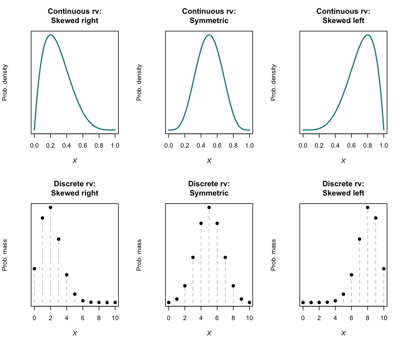
FIGURE 5.3: Examples of right-skewed (left panels), symmetric (centre panels) and left-skewed (right panels) distributions. Top: continuous random variable. Bottom: discrete random variable.
Example 5.21 (Skewness) Consider the random variable \(X\) in Example 5.15, where \(f_X(x) = x(2 - x)\) for \(0 < x < 2\). From that example, \(\operatorname{E}[X] = \mu'_1 = 1\) and \(\operatorname{E}[X^2] = \mu'_2 = 6/5\). Then, \[ \mu_3 = \int_0^2 (x - 1)^3\times 3x(2 - x)/4 \,dx = 0, \] so that the skewness in Eq. (5.2) will be zero. This is expected, since the distribution is symmetric (Fig. 5.4).
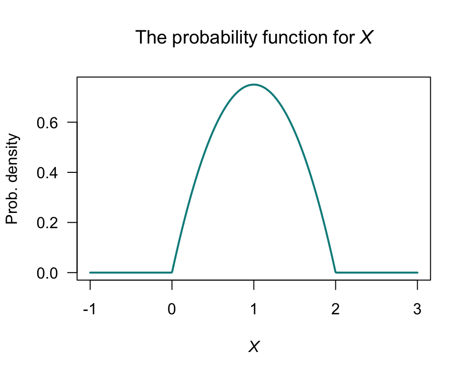
FIGURE 5.4: The probability density function for \(X\).
Example 5.22 (Skewness) Consider the random variable \(Y\) with PMF \[ p_Y(y) = \begin{cases} 0.2 & \text{for $y = 5$};\\ 0.3 & \text{for $y = 6$};\\ 0.5 & \text{for $y = 7$}. \end{cases} \] Then \[ \mu'_1 = \operatorname{E}[Y] = (5\times 0.2) + (6\times 0.3) + (7\times 0.5) = 6.3. \] Likewise, \[\begin{align*} \mu_2 &= \operatorname{E}\big[(y - 6.3)^2 \big] = (5 - 6.3)^2\times 0.2 + (6 - 6.3)^2\times 0.3 + (7 - 6.3)^2\times 0.5 = 0.61;\quad{\text{and}}\\ \mu_3 &= \operatorname{E}\big[(y - 6.3)^3 \big] = (5 - 6.3)^3\times 0.2 + (6 - 6.3)^3\times 0.3 + (7 - 6.3)^3\times 0.5 = -0.276. \end{align*}\] Hence, the skewness is \[ \gamma_1 = \frac{\mu_3}{\mu_2^{3/2}} = \frac{-0.276}{0.61^{3/2}} = -0.579\dots, \] so the distribution has slight negative skewness.
5.5.3 Kurtosis
Another description of a distribution is kurtosis, which measures the heaviness of the tails in a distribution; that is, how much of the probability of the random variable \(X\) is concentrated in the extreme values of \(X\). This is related to the fourth central moment. Again, finding the appropriate expected value of a normalised version of the random variable (i.e., with mean zero and variance one) is preferred. That is, the definition of kurtosis finds the appropriate expected value of \((X - \mu)/\sigma\) rather than of \(X\) directly.
Definition 5.9 (Kurtosis) The kurtosis of a random variable \(X\) with mean \(\mu = \operatorname{E}[X]\) and variance \(\sigma^2 = \operatorname{var}[X]\) is defined as \[ \text{kurtosis} = \operatorname{E}\left[\left(\frac{X-\mu}{\sigma}\right)^4\right] = \frac{\mu_4}{\mu^2_2}. \] The excess kurtosis of the distribution of a random variable is defined as \[\begin{equation*} \gamma_2 = \frac{\mu_4}{\mu^2_2} - 3. \end{equation*}\] The excess kurtosis definition defines the excess kurtosis compared to a bell-shaped (normal distribution), which has an excess kurtosis of zero.
Excess kurtosis is so commonly used that is often referred to as ‘kurtosis’.
One way to understand kurtosis (from Moors (1986)) is to first define \(Z = (X - \mu)/\sigma\); then the kurtosis is, from Def. 5.9, \(\operatorname{E}[Z^4]\), and \(\operatorname{E}[Z] = 0\) and \(\operatorname{var}[X] = 1\). Also observe that since \(\operatorname{var}[X] = \operatorname{E}[X^2] - \operatorname{E}[X]^2\) (the definition of variance), we can write \[\begin{equation} \operatorname{E}[X^2] = \operatorname{var}[X] + \operatorname{E}[X]^2. \tag{5.3} \end{equation}\] Then, the kurtosis is \[\begin{align*} \operatorname{E}[Z^4] &= \operatorname{var}[Z^2] + \operatorname{E}[Z^2]^2\quad\text{(using Eq.~(\ref{eq:VarianceRearranged}))}\\ &= \operatorname{var}[Z^2] + \left[ \operatorname{var}[Z] + \operatorname{E}[Z]^2\right]^2\quad\text{(using Eq.~(\ref{eq:VarianceRearranged}) again)}\\ &= \operatorname{var}[Z^2] + (1 + 0)^2 \\ &= \operatorname{var}[Z^2] + 1. \end{align*}\] Thus, the kurtosis is related to the variance of \(Z^2\) (not \(Z\)) about the mean. That is, kurtosis emphasises the probability function in the extremes of the random variable.
Large values of kurtosis corresponds to greater proportion of the distribution in the tails. Then (see Fig. 5.5):
- distributions with negative excess kurtosis are called platykurtic. These distribution have fewer, or less extreme, observations in the tail compared to the normal distribution (‘thinner tails’). Examples include the Bernoulli distribution (Sect. 6.3).
- distributions with positive excess kurtosis are called leptokurtic. These distribution have more, or more extreme, observations in the tail compared to the normal distribution (‘fatter tails’). Examples include the exponential distribution (Sect. 7.4) and Poisson distributions (Sect. 6.7).
- distributions with zero excess kurtosis are called mesokurtic. The normal distribution (Sect. 7.3) is the obvious example.
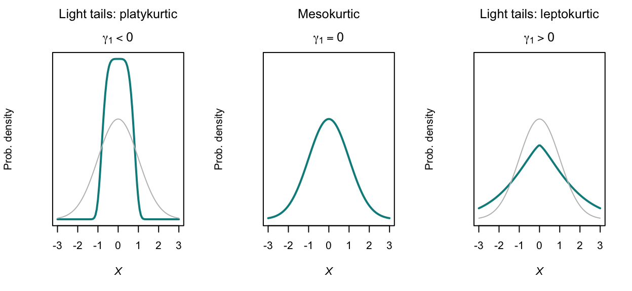
FIGURE 5.5: Kurtosis for three distributions plotted from \(x = -3\) to \(x = +3\); all plots have mean of \(0\), variance of \(1\) and are symmetric. The grey line shows the middle distribution as a reference, with \(\gamma_1 = 0\) (zero excess kurtosis).
Example 5.23 (Uses of skewness and kurtosis) Monypenny and Middleton (1998b) and Monypenny and Middleton (1998a) use the skewness and kurtosis to analyse wind gusts at Sydney airport.
Example 5.24 (Uses of skewness and kurtosis) Galagedera et al. (2002) used higher moments in a capital analysis pricing model for Australian stock returns.
Example 5.25 (Skewness and kurtosis) Consider the discrete random variable \(U\) from Example 5.1. The raw moments are \[\begin{align*} \mu'_r = \operatorname{E}[U^r] &= \sum_{u = -1, 0, 1} u^r \frac{u^2 + 1}{5} \\ &= (-1)^r \frac{ (-1)^2 + 1}{5} + (0)^r \frac{ (0)^2 + 1}{5} + (1)^r \frac{ (1)^2 + 1}{5} \\ &= \frac{2(-1)^r}{5} + 0 + \frac{2}{5} \\ &= \frac{2}{5}[ (-1)^r + 1] \end{align*}\] for the \(r\)th raw moment. Then, \[\begin{align*} \operatorname{E}[X] &= \mu'_1 = \frac{2}{5}[ (-1)^1 + 1 ] = 0;\\ \operatorname{E}[X^2] &= \mu'_2 = \frac{2}{5}[ (-1)^2 + 1 ] = 4/5;\\ \operatorname{E}[X^3] &= \mu'_3 = \frac{2}{5}[ (-1)^3 + 1 ] = 0;\\ \operatorname{E}[X^4] &= \mu'_4 = \frac{2}{5}[ (-1)^4 + 1 ] = 4/5. \end{align*}\] Since \(\operatorname{E}[U] = 0\), then the \(r\)th central and raw moments are the same: \(\mu'_r = \mu_r\). Notice that once the initial computations to find \(\mu'_r\) are complete, the evaluation of any raw moment is simple.
The skewness is \[ \gamma_1 = \frac{\mu_3}{\mu_2^{3/2}} = \frac{0}{(4/5)^{3/2}} = 0, \] so the distribution is symmetric. The excess kurtosis is \[ \gamma_2 = \frac{\mu_4}{\mu_2^2} -3 = \frac{4/5}{(4/5)^2} -3 = -7/4, \] so the distribution is platykurtic.
5.6 Moment generating functions
5.6.1 Introduction
By themselves, the mean, variance, skewness and kurtosis do not completely describe a distribution; many different distributions can be found having a given mean, variance, skewness and kurtosis. However, in general, all the moments of a distribution together define the distribution. This leads to the idea of a moment generating function.
Suppose I asked you to draw the probability density function of a random variable \(X\), with \(\operatorname{E}[X] = 2\). Any of the six distributions in Fig. 5.6 meet this (first moment) criterion, so this information is not sufficient to uniquely define a distribution.
So, suppose a second criterion is added: in addition, we require \(\operatorname{var}[X] = 1\). Any of the first five distributions in Fig. 5.6 meet these two criteria (based on the first two moments), so again this information is not sufficient to uniquely define a distribution.
Suppose a third criterion is added: the distribution must be symmetric. Any of the top four distributions in Fig. 5.6 meet these three criteria (based on the first three moments); again, this information is not sufficient to uniquely define a distribution.
Suppose a fourth criterion is added: the distribution must have zero excess kurtosis. Either of the top two distributions in Fig. 5.6 meet these four criteria (based on the first four moments); again, this information is not sufficient to uniquely define a distribution.
In general, all the moments of a distribution are needed to uniquely define a distribution. However, computing all (or even many) moments of a distribution is usually very tedious. For this reason, the moment generating function (or MGF) is now introduced, a function that encapsulates all the moments of a distribution.
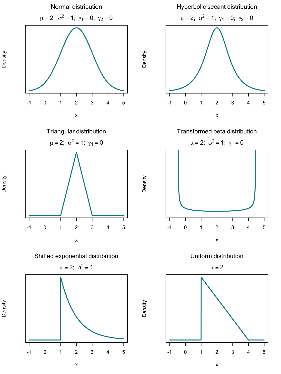
FIGURE 5.6: Six distributions, all with mean \(1\). All distributions apart from the bottom right have variance \(1\). The top four distributions are symmetric (i.e., \(\gamma_1 = 0\)); the top two distributions have zero excess kurtosis (i.e., \(\gamma_2=0\)).
5.6.2 Definition
So far, the distribution of a random variable has been described using a probability function or a distribution function. Sometimes, however, working with a different representation is useful (for example, see Sect. 9.4).
In this section, the moment generating function is used to represent the distribution of the probabilities of a random variable. As the name suggests, this function can be used to generate any moment of a distribution. Other uses of the moment generating function are seen later (see Sect. 9.4).
Definition 5.10 (Moment generating function (MGF)) The moment generating function (or MGF) \(M_X(t)\) of the random variable \(X\) defined over a range \(\mathcal{R}_X\) is denoted \(M_X(t)\), and defined as \[ M_X(t) = \operatorname{E}\big[\exp(tX)\big], \] provided the expectation exists for values of \(t\) in some interval that includes \(t = 0\).
When \(X\) is a discrete random variable, \[ M_X(t) = \operatorname{E}\big[\exp(tX)\big] = \sum_{x\in \mathcal{R}_X} \exp(tx)\, p_X(x). \] When \(X\) is a continuous random variable, \[ M_X(t) = \operatorname{E}\big[\exp(tX)\big] = \int_{-\infty}^\infty \exp(tx)\, f_X(x)\, dx. \] When \(X\) is a mixed random variable with probability mass function \(p_X(x)\) and probability density function \(f_X(x)\), \[ M_X(t) = \operatorname{E}\big[\exp(tX)\big] = \sum_{x\in \mathcal{R}_X} \exp(tx)\, p_X(x) + \int_{-\infty}^{\infty} \exp(tx)\, f_X(x)\, dx, \] where \(\mathcal{R}_X\) is the set of values having positive probability mass.
The MGF may not converge to a finite value for all values of \(t\), so may not be defined everywhere. Note that the MGF always exists for \(t = 0\); in fact \(M_X(0) = 1\).
Provided the MGF is defined for some values of \(t\) other than zero, it uniquely defines a probability distribution, and we can use it to easily generate the moments of the distribution, as described in Theorem 5.7.
Moment generating functions are related to Laplace transformations.
Example 5.26 (Moment generating function) Consider the random variable \(X\) with PDF \[ f_X(x) = \exp(-x) \qquad \text{for $x > 0$}. \] The MGF is \[\begin{align*} M_X(t) = \operatorname{E}[\exp(tX)] &= \int_0^\infty \exp(tx)\,\exp(-x)\, dx \\ &= \int_0^\infty \exp\{ x(t - 1) \}\, dx \\ &= (1 - t)^{-1} \end{align*}\] provided \(t - 1 < 0\); that is, for \(t < 1\) (which includes \(t = 0\)). If \(t > 1\), the integral does not converge. For example, if \(t = 2\), \[ M_X(t) = \int_0^\infty \exp(x)\, dx \] which does not converge.
Example 5.27 (MGF for die rolls) Consider the PMF of \(X\), the outcome of tossing a fair die (Example 5.13). The MGF of \(X\) is \[\begin{align*} M_X(t) &= \operatorname{E}[\exp(tX)] = \sum_{x = 1}^6 \exp(tx)\, p_X(x)\\ &= \frac{1}{6}\left( \exp t + \exp(2t) + \exp(3t) + \exp(4t) + \exp(5t) + \exp(6t)\right), \end{align*}\] which exists for all values of \(t\).
Example 5.28 (MGF does not exist) Consider the Cauchy distribution with the PDF \[ f_X(x) = \frac{1}{\pi(1 + x^2)}, \] defined over \(x\in\mathbb{R}\). The moment generating function is \[ \operatorname{E}[\exp(tX)] = \int_{-\infty}^{\infty} \exp(tx)\frac{1}{\pi(1 + x^2)}\,dx. \] This integrand does not converge unless \(t = 0\).
For example, consider \(t > 0\): as \(x\to\infty\), we see \(\exp(tx)\to\infty\), while \(1/(1 + x^2)\to 0\) quite slowly; the integrand diverges (see Fig. 5.7 (left panel) for an example when \(t = 1\)).
Now consider \(t < 0\): as \(x\to-\infty\), we see \(\exp(tx)\to\infty\), while \(1/(1 + x^2)\to 0\) quite slowly; the integrand again diverges (see Fig. 5.7 (right panel) for an example when \(t = -1\)).
The integral only converges for \(t = 0\). The definition for the MGF states that the MGF exists ‘provided the expectation exists for values of \(t\) in some interval that includes \(t = 0\)’. This is not the case: the integral exists only for \(t = 0\). The MGF does not exist for the Cauchy distribution.
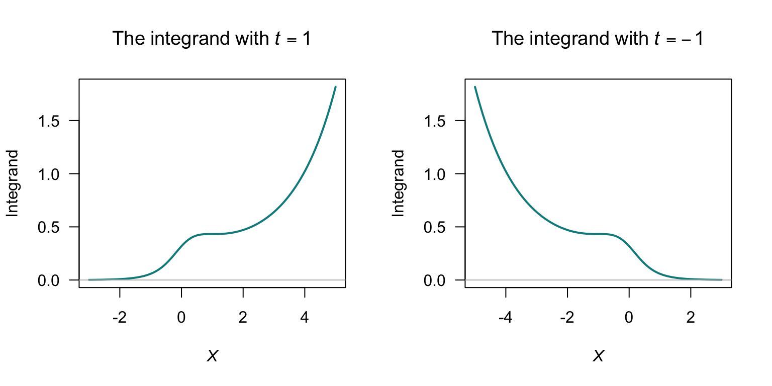
FIGURE 5.7: The MGF cannot be computed, as the integrand diverges for \(t > 0\) (left panel) and for \(t < 0\) (right panel).
5.6.3 Using the MGF to generate moments
Replacing \(\exp(xt)\) by its series expansion (App. B) in the definition of the MGF for a discrete random variable \(X\) gives \[\begin{align*} M_X(t) & = {\sum_x} \left(1 + xt + \frac{x^2t^2}{2!} + \dots\right) p_X(x)\\ & = 1 + \mu'_1t + \mu'_2 \frac{t^2}{2!} +\mu'_3 \frac{t^3}{3!} + \dots \end{align*}\] Then, the \(r\)th moment of a distribution about the origin is seen to be the coefficient of \(t^r/r!\) in the series expansion of \(M_X(t)\): \[\begin{align*} \frac{d M_X(t)}{dt} & = \sum_x x\,\exp(xt) p_X(x)\\ \frac{d^2 M_X(t)}{dt^2} & = \sum_x x^2\,\exp(xt) p_X(x), \end{align*}\] and, in general, for each positive integer \(r\): \[ \frac{d^r M_X(t)}{dt^r} = \sum_x x^r \exp(xt)\, p_X(x). \] On setting \(t = 0\), \[\begin{align*} \left.\frac{d M_X(t)}{dt}\right|_{t = 0} &= \operatorname{E}[X]\\ \left.\frac{d^2M_X(t)}{dt^2}\right|_{t = 0} &= \operatorname{E}[X^2]. \end{align*}\] (The notation to the left means to evaluate the expression at \(t = 0\).) In general, for each positive integer \(r\), \[\begin{equation} \left.\frac{d^r M_X(t)}{dt^r}\right|_{t = 0} = \operatorname{E}[X^r]. \end{equation}\] (Sometimes, \(d^r M_X(t)/dt^r\) evaluated at \(t = 0\) is written as \(M^{(r)}(0)\) for brevity.) This result is summarised in the following theorem.
Theorem 5.7 (Moments) The \(r\)th moment \(\mu'_r\) of the distribution of the random variable \(X\) about the origin is given by either
- the coefficient of \(t^r/r!, r = 1, 2, 3,\dots\) in the power series expansion of \(M_X(t)\); or
- \(\displaystyle \mu'_r = \left.\frac{d^rM(t)}{dt^r}\right|_{t = 0}\) where \(M_X(t)\) is the MGF of \(X\).
Example 5.29 (Mean and variance from a MGF) Continuing Example 5.26, the mean and variance of \(X\) can be found from the MGF. To find the mean, first find \[ \frac{d}{dt}M_X(t) = (1 - t)^{-2}. \] Setting \(t = 0\) gives the mean as \(\operatorname{E}[X] = 1\). Likewise, \[ \frac{d^2}{dt^2}M_X(t) = 2(1 - t)^{-3}. \] Setting \(t = 0\) gives \(\operatorname{E}[X^2] = 2\). The variance is therefore \(\operatorname{var}[X] = 2 - 1^2 = 1\).
Once the moment generating function has been computed, raw moments can be computed using \[ \operatorname{E}[X^r] = \mu'_r = \left.\frac{d^r}{dt^r} M_X(t)\right|_{t = 0}. \]
5.6.4 Some useful results
The moment generating function can be used to derive the distribution of a function of a random variable (see Sect. 9.4). The following theorems are valuable for this task.
Theorem 5.8 (MGF of linear combinations) If the random variable \(X\) has MGF \(M_X(t)\) and \(Y = aX + b\) where \(a\) and \(b\) are constants, then the MGF of \(Y\) is \[ M_Y(t) = \operatorname{E}\big[\exp\{t(aX + b)\}\big] = \exp(bt) M_X(at). \]
Theorem 5.9 (MGF of independent rvs) If \(X_1\), \(X_2\), \(\dots\), \(X_n\) are \(n\) independent random variables, where \(X_i\) has MGF \(M_{X_i}(t)\), then the MGF of \(Y = X_1 + X_2 + \cdots X_n\) is \[ M_Y(t) = \prod_{i = 1}^n M_{X_i}(t). \]
Proof. The proofs are left as an exercise.
Note that in the special case when all the random variables are independently and identically distributed in Theorem 5.9, we have \[ M_Y(t) = [M_{X_i}(t)]^n. \]
Example 5.30 (MGF of linear combinations) Consider the random variable \(X\) with probability mass function \[ p_X(x) = 2(1/3)^x \qquad \text{for $x = 1, 2, 3, \dots$}. \] The MGF of \(X\) is \[\begin{align*} M_X(t) &= \sum_{x: p(x) > 0} \exp(tx)\, p_X(x) \\ &= \sum_{x = 1}^\infty \exp(tx)\, 2(1/3)^x \\ &= 2\sum_{x = 1}^\infty (\exp(t)/3)^x \\ &= 2\left\{ \frac{\exp(t)}{3} + \left(\frac{\exp(t)}{3}\right)^2 + \left(\frac{\exp(t)}{3}\right)^3 + \dots\right\} \\ &= \frac{2\exp(t)}{3 - \exp(t)} \end{align*}\] where \(\sum_{y = 1}^\infty a^y = a/(1 - a)\) for \(a < 1\) has been used (App. B); here \(a = \exp(t)/3\).
Next consider finding the MGF of \(Y = (X - 2)/3\). From Theorem 5.8 with \(a = 1/3\) and \(b = -2/3\), \[ M_Y(t) = \exp(-2t/3) M_X(t/3) = \frac{2\exp\{(-t)/3\}}{3 - \exp(t/3)}. \] In practice, rather than identify \(a\) and \(b\) and remember Theorem 5.8, problems like this are best solved directly from the definition of the MGF: \[\begin{align*} M_Y(t) = \operatorname{E}[\exp(tY)] &= \operatorname{E}[\exp\{t(X - 2)/3\}]\\ &= \operatorname{E}[\exp\{tX/3 - 2t/3\}]\\ &= \exp(-2t/3) M_X(t/3) \\ &= \frac{2\exp\{(-t)/3\}}{3 - \exp(t/3)}. \end{align*}\]
5.6.5 Recovering the distribution from the MGF
The MGF (if it exists) completely determines the distribution of a random variable hence, given a MGF, deducing the probability function should be possible. For some distributions, the PDF cannot be written in closed form (so the PDF can only be evaluated numerically; for example, see Sect. 8.3), but the MGF is relatively simple to write down.
For a discrete random variable \(X\), the MGF is defined as \[\begin{equation} M_X(t) = \operatorname{E}[\exp(tX)] = \sum_X \exp(tx) p_X(x) \tag{5.4} \end{equation}\] for \(X\) discrete with PMF \(p_X(x)\). This can be expressed as \[ M_X(t) = \exp(t x_1) p_X(x_1) + \exp(t x_2)p_X(x_2) + \dots \] and so the probability function \(p_X(x)\) of \(X\) can be deduced from the MGF.
Example 5.31 (Distribution from the MGF) Suppose a discrete random variable \(D\) has the MGF \[ M_D(t) = \frac{1}{3} \exp(2t) + \frac{1}{6}\exp(3t) + \frac{1}{12}\exp(6t) + \frac{5}{12}\exp(7t). \] Then, by the definition of the MGF in the discrete case given above, the coefficient of \(t\) in the exponential indicates values of \(D\), and the coefficient indicates the probability of that value of \(Y\): \[\begin{align*} M_D(t) &= \overbrace{\frac{1}{3} \exp(2t)}^{D = 2} + \overbrace{\frac{1}{6}\exp(3t)}^{D = 3} + \overbrace{\frac{1}{12}\exp(6t)}^{D = 6} + \overbrace{\frac{5}{12}\exp(7t)}^{D = 7}\\ &= \Pr(D = 2)\exp(2t) + \Pr(D = 3)\exp(3t) + \\ & \qquad \Pr(D = 6)\exp(6t) + \Pr(D = 7)\exp(7t). \end{align*}\] So the PMF is \[ p_D(d) = \begin{cases} 1/3 & \text{for $d = 2$};\\ 1/6 & \text{for $d = 3$};\\ 1/12 & \text{for $d = 6$;}\\ 5/12 & \text{for $d = 7$}. \end{cases} \] (Of course, you can check by computing the MGF for \(D\) from the probability mass function found above.)
Sometimes, using the results in App. B can be helpful.
Example 5.32 (Distribution from the MGF) Consider the MGF \[ M_X(t) = \frac{\exp(t)}{3 - 2\exp(t)}. \] To find the corresponding probability function, one approach is to write the MGF as \[ M_X(t) = \frac{\exp(t)/3}{1 - 2\exp(t)/3}. \] This is the sum of a geometric series (Eq. (B.5)): \[ a + ar + ar^2 + \ldots + ar^{n - 1} \rightarrow \frac{a}{1 - r} \text{ as $n \rightarrow \infty$}, \] where \(a = \exp(t)/3\) and \(r = 2\exp(t)/3\). Hence the MGF can be expressed as \[ \frac{1}{3}\exp(t) + \frac{1}{3}\left(\frac{2}{3}\right) \exp(2t) + \frac{1}{3}\left(\frac{2}{3}\right)^2 \exp(3t) + \dots \] so that the probability function can be deduced as \[\begin{align*} \Pr(X = 1) &= \frac{1}{3};\\ \Pr(X = 2) &= \frac{1}{3}\left(\frac{2}{3}\right);\\ \Pr(X = 3) &= \frac{1}{3}\left(\frac{2}{3}\right)^2, \end{align*}\] or, in general, \[ p_x(x) = \frac{1}{3}\left( \frac{2}{3}\right)^{x - 1}\quad\text{for $x = 1, 2, 3, \dots$}. \] (Later, this will be identified as a geometric distribution.)
For a continuous random variable \(X\), the approach is more involved, and so is delayed until Sect. 5.7.2.
5.7 MGF-like functions*
The moment generating function is one member of a family of transformation that encode information about a distribution. Two closely related transforms are the cumulant generating function and the characteristic function. Each has properties that make it preferable to the MGF in certain situations.
5.7.1 Cumulant generating function*
The cumulant generating function is closely related to the MGF.
Definition 5.11 (Cumulant generating function) The cumulant generating function (CGF) of a random variable \(X\) is the natural logarithm of the MGF, wherever the MGF exists: \[ K_X(t) = \log M_X(t). \] Since \(M_X(0) = 1\), then \(K_X(0) = 0\).
The CGF can be used to generate the cumulants of a distributions, which are the coefficients in the Maclaurin series for \(K_X(t)\): \[ K_X(t) = \sum_{r=1}^{\infty} \kappa_r \frac{t^r}{r!}. \] The \(r\)-th cumulant is \[ \kappa_r = K_X^{(r)}(0) = \left.\frac{d^r}{dt^r} K_X(t)\right|_{t=0} \] The first four cumulants have direct interpretations (where \(\mu_r = E[(X - \mu)^r]\) denotes the \(r\)-th central moment):
- The first cumulant \(\kappa_1\), is \(\mu_1' = \operatorname{E}[X]\) (the mean).
- The second cumulant, \(\kappa_2\), is \(\mu_2' - (\mu_1')^2 = \operatorname{var}[X]\) (the variance).
- The third cumulant, \(\kappa_3\), is \(\mu_3\) (the third central moment) (related to skewness).
- The fourth cumulant, \(\kappa_4\), is \(\mu_4 - 3\mu_2^2\) (the fourth central moment minus \(3\sigma^4\)), related to excess kurtosis.
The standardised skewness and excess kurtosis can be written neatly in terms of cumulants: \[ \gamma_1 = \frac{\kappa_3}{\kappa_2^{3/2}}, \qquad \gamma_2 = \frac{\kappa_4}{\kappa_2^2}. \]
The most important property of cumulants is their additivity under convolution. If \(X\) and \(Y\) are independent, then for all \(r\): \[ \kappa_r(X + Y) = \kappa_r(X) + \kappa_r(Y). \] This follows from \(K_{X + Y}(t) = K_X(t) + K_Y(t)\) (which itself follows from \(M_{X + Y}(t) = M_X(t)\cdot M_Y(t)\) for independent random variables \(X\) and \(Y\)).
This additivity is the reason cumulants are often more convenient than moments when working with sums of independent random variables; adding moments requires the binomial theorem and rapidly becomes algebraically messy, while adding cumulants is trivial.
Example 5.33 (Cumulants) Supose the random variable \(X\) has the probability mass function \[ p_X(x) = \frac{\exp(-\lambda)\lambda^x}{x!}\quad\text{for $x = 0, 1, 2, \dots$}. \] The MGF is \[\begin{align*} M_X(t) &= \sum_{x = 0}^\infty \exp(t x) \frac{\exp(-\lambda)\lambda^x}{x!}\\ &= \exp(-\lambda) \sum_{x = 0}^\infty \frac{\left(\exp(t)\lambda\right)^x}{x!}\\ &= \exp(-\lambda) \exp(\lambda \exp t)\\ &= \exp(\lambda(\exp t - 1)) \end{align*}\] where Eq.~(B.8) has been used. Thus, \[ K_X(t) = \log M_X(t) = \lambda(\exp t - 1). \] Differentiating \(r\) times and evaluating at \(t = 0\) gives \(\kappa_r = \lambda\) for all \(r \geq 1\). All cumulants of the distribution are \(\lambda\).
5.7.2 Characteristic function*
The CGF inherits the main limitation of the MGF: it may not exist. For heavy-tailed distributions such as the Cauchy or Pareto, the MGF does not exist in any neighbourhood of zero, and hence neither does the CGF. For such distributions the characteristic function is required.
Definition 5.12 (Characteristic function) The characteristic function replaces \(t\) in the MGF with \(it\) (where \(i = \sqrt{-1}\,\)), giving \[ \varphi_X(t) = \operatorname{E}[\exp(itX)] = \operatorname{E}[\cos tX] + i\, \operatorname{E}[\sin tX] \quad\text{for $t \in \mathbb{R}$}. \] Because \(|\exp(itX)| = 1\) for all real \(t\) and \(X\), the expectation always exists; no moment conditions are required.
For a continuous random variable \(X\) with density \(f_X(x)\): \[ \varphi_X(t) = \int_{-\infty}^{\infty} \exp(itx) f_X(x)\, dx, \] which is the Fourier transform of the density. For a discrete random variable \(X\): \[ \varphi_X(t) = \sum_x \exp(itx) p_X(x). \] The characteristic function is sometimes preferred over the MGF and CGF because it always exists, (i.e., \(\varphi_X(t)\) is well-defined and bounded for every distribution), and it is unique for every distribution (i.e., if \(\varphi_X(t) = \varphi_Y(t)\) for all \(t \in \mathbb{R}\), then \(X\) and \(Y\) have the same distribution). The uniqueness property is the analogue of the uniqueness theorem for MGFs, but holds without any moment restrictions.
When the MGF exists in a neighbourhood of zero, the characteristic function is obtained by formally substituting \(t \to -it\): \[ \varphi_X(t) = M_X(it). \] That is, the characteristic function is the MGF evaluated on the imaginary axis. When the MGF does not exist (heavy-tailed distributions), the characteristic function still exists and carries all distributional information.
Example 5.34 (Characteristic function) Consider the random variable \(X\) in Example 5.33. The characteristic function is \[ \varphi_X(t) = \exp\!\left[\lambda(\exp(it) - 1)\right]. \] Compare with the MGF \(M_X(t) = \exp[\lambda(\exp t - 1)]\): the substitution \(t \to it\) is all that is needed.
The characteristic function always exists and is unique for every distribution. As a result, the characteristic function can be used to recover the PDF for a continuous random variable (also see Sect. 5.6.5 for recovering the PMF for a discrete random variable).
Suppose the continuous random variable \(X\) has the characteristic function \(\varphi_X(t)\). Then the probability density function is (see Abramowitz and Stegun (1964), 26.1.10) \[\begin{equation} f_X(x) = \frac{1}{2\pi} \int_{-\infty}^{\infty} \varphi_X(t) \exp(-itx)\, dt, \tag{5.5} \end{equation}\] where \(i = \sqrt{-1}\). While Eq. (5.5) recovers the probability density function in theory, often the integrals produced are difficult to evaluate.
Example 5.35 (Distribution from the MGF) In Example 5.26, an MGF was found for a distribution: \[ M_X(t) = \frac{1}{1 - t}. \] The characteristic function is \[ \varphi_X(t) = \frac{1}{1 - it}. \] Using Eq. (5.5), the density function can be recovered as \[\begin{align*} f_X(x) &= \frac{1}{2\pi} \int_{-\infty}^{\infty} \frac{1}{1 - it} \exp(-itx)\, dt,\\ &= \frac{1}{2\pi} \int_{-\infty}^{\infty} \frac{1 + it}{1 + t^2} \left( \cos(tx) - i\sin(tx) \right) \, dt \end{align*}\] multiplying the top and bottom of the fraction by the complex conjugate \(1 + it\). By symmetry, the imaginary parts must integrate to zero. Then, since \(f_X(x)\) is real, take the real parts: \[\begin{align*} f_X(x) &= \frac{1}{2\pi} \int_{-\infty}^{\infty} \frac{\cos(tx) + t\sin(tx)}{1 + t^2} \, dt. \end{align*}\] This is not an easy integral to complete without using complex analysis; using tabulated integral results (Sect. C.5), we obtain \[ f_X(x) = \exp(-x), \] the original density function in Example 5.26.
In practice, using Eq. (5.5) can become tedious or intractable for producing a closed form expression for the PDF. However, Eq. (5.5) has been used in practice to compute numerical values of the probability density function. For example, Dunn and Smyth (2008) used Eq. (5.5) to evaluate the PDF for the Tweedie distributions (Dunn and Smyth 2001), which includes the compound Poisson–gamma distributions as a special case (Sect. 8.3). The Tweedie distributions (in general) have no closed for the PDF, but they do have a simple MGF.
The MGF, when it exists, is most useful when and moments are the main interest. The CGF is most useful when working with cumulants, or sums of independent random variables. The characteristic function is useful when dealing with heavy-tailed distributions (as it always exist).
5.8 Numerical approaches
Some distributions cannot be written in closed form (i.e., a neat function of standard mathematical functions), which makes (for example) evaluation of probability and computation of means difficult. In these cases, numerical methods, such as numerical integration, may be needed.
Consider the random variable \(X\) with density function
\[
f_X(x) = \frac{c}{\sqrt{x}}\exp( -x - \sqrt{2x}\,)\quad \text{for $x > 0$}.
\]
for some normalising constant \(c\).
This density function has no closed form, and the value of \(c\) cannot be found via integration.
However, the value of \(c\) could be found using numerical integration in R using integrate():
### Define the function, without the constant term
g <- function(x){
  ifelse(x > 0,
         x^(-0.5) * exp(-x - sqrt(2 * x)), # When x > 0
         0)                                # When x <= 0
}

### Integrate between 0 and infinity:
#\n adds a "new line"
Const <- 1 / integrate(g,
                       lower = 0,
                       upper = Inf)$value
cat("The value of  c  is about", round(Const, 4), "\n")
#> The value of  c  is about 1.0784

# So now define f(x):
f <- function(x){
  ifelse(x > 0,
         x^(-0.5) * exp(-x - sqrt(2 * x)) * Const,  # When x > 0
         0)                                         # When x <= 0
}
That is, \(c = 1.0784\dots\). The distribution function can be found:
F <- function(x){
  F <- array(dim = length(x) )
  for (i in 1:length(x)){
    F[i] <- integrate( f,
                       lower = 0,
                       upper = x[i])$value
  }
  return(F)
}
So now the density and the distribution function can be plotted (Fig. 5.8):
### Make room for two plots side-by-side
par( mfrow = c(1, 2))

### Evaluate over these values of x
x <- seq(0.01, 2,
         length = 1000)

# Define the function
f2 <- function(x) { g(x) * Const}

# Plot
curve(f2,
      from = 0.01, to = 2,
      las = 1, lwd = 3,
      main = "Density function",
      xlab = expression(italic(x)),
      ylab = "Density fn.")
curve(F,
      from = 0.00001, to = 2,
      type = "l", ylim = c(0, 1),
      las = 1, lwd = 3,
      main = "Distribution function",
      xlab = expression(italic(x)),
      ylab = "Distribution fn.")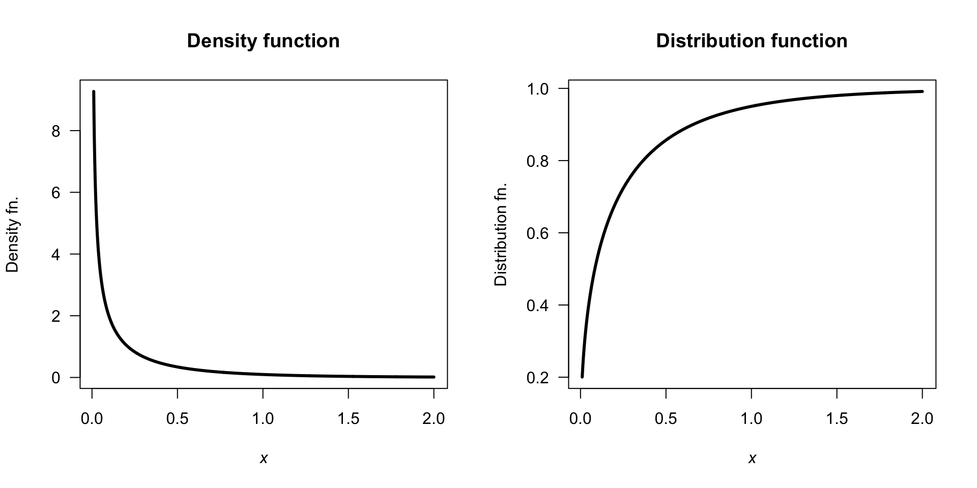
FIGURE 5.8: The density function (left) and distribution function (right) of a distribution that cannot be expressed in closed form.
Probabilities can then be computed; for example, we can find \(\Pr(X > 0.5)\):
integrate(f,
          lower = 0.5,
          upper = Inf)
#> 0.1433935 with absolute error < 4.4e-06
And the expected value of \(X\), \(\operatorname{E}[X]\), can be found:
f_Expected <- function(x){
  x * f(x)
}
integrate(f_Expected,
          lower = 0,
          upper = Inf)
#> 0.2374324 with absolute error < 2.1e-07
5.9 Exercises
Selected answers appear in Sect. F.4.
Exercise 5.1 The PDF for the random variable \(Y\) is defined as \[ f_Y(y) = 2y + k \qquad \text{for $1\le y \le 2$}. \]
- Find the value of \(k\).
- Plot the PDF of \(Y\).
- Compute \(\operatorname{E}[Y]\).
- Compute \(\operatorname{var}[Y]\).
- Compute \(\Pr(Y > 1.5)\).
Exercise 5.2 The PDF for the random variable \(X\) is defined as \[ f_X(x) = \begin{cases} 2(x + 1)/ 3 & \text{for $-1\le x \le 0$};\\ (2 - x)/ 3 & \text{for $0 < x \le 2$}. \end{cases} \]
- Plot the PDF of \(X\).
- Compute \(\operatorname{E}[X]\).
- Compute \(\operatorname{var}[X]\).
- Compute \(\Pr(X > 0)\).
Exercise 5.3 The random variable \(T\) has the density function \[ f_T(t) = \begin{cases} 1/2 & \text{for $0 < t < 1$};\\ 2 - t & \text{for $1 \le t < 2$}. \end{cases} \]
- Plot the PDF of \(T\).
- Compute \(\operatorname{E}[T]\).
- Compute \(\operatorname{var}[T]\).
- Find and plot the distribution function of \(T\).
- Compute \(\Pr(T \le 1)\).
Exercise 5.4 The random variable \(Z\) has the density function \[ f_Z(z) = \begin{cases} 1 - z & \text{for $0 < z < 1$};\\ z - 2 & \text{for $2 < z < 3$}. \end{cases} \]
- Plot the PDF of \(Z\).
- Compute \(\operatorname{E}[Z]\).
- Compute \(\operatorname{var}[Z]\).
- Find and plot the distribution function of \(Z\).
- Compute \(\Pr(Z > 2 \mid Z > 1)\).
Exercise 5.5 The PMF for the random variable \(D\) is defined as \[ p_D(d) = \begin{cases} 1/2 & \text{for $d = 1$};\\ 1/4 & \text{for $d = 2$};\\ k & \text{for $d = 3$}, \end{cases} \] for a constant \(k\).
- Plot the probability mass function.
- Compute the mean and variance of \(D\).
- Find the MGF for \(D\).
- Compute the mean and variance of \(D\) from the MGF.
- Compute \(\Pr(D < 3)\).
Exercise 5.6 The PMF for the random variable \(Z\) is defined as \[ p_Z(z) = c/z^2 \qquad \text{for $z = 1, 2, 3, 4$} \] for a constant \(c\).
- Plot the probability mass function.
- Compute the mean and variance of \(Z\).
- Find the MGF for \(Z\).
- Compute the mean and variance of \(Z\) from the MGF.
- Compute \(\Pr(Z \ge 2)\).
Exercise 5.7
An ecologist records fish biomass \(X\) at sampling sites. Suppose \(\Pr(X = 0) = 0.6\) and \[ f_X(x \mid X > 0) = exp(-x)\quad\text{for $x > 0$)}. \]
- Find the expected biomass.
- Find the variance of the the biomass.
- Find the MGF of \(X\).
- Compute the mean and variance of \(X\) from the MGF.
Exercise 5.8
Suppose the true daily rainfall \(X\) follows a distribution with probability function \(f_X(x) = \exp( -x/20)/20\). A rainfall gauge records \[ R = \begin{cases} 0 & \text{for $X < 0.1$}\\ X & \text{for $0.1 \le X\le 70$}\\ 70 & \text{for $X>70$}. \end{cases} \]
- Find the expected value of \(R\).
- Find the variance of \(R\).
- Find the MGF of \(X\), and write down the expression for evaluating the MGF of \(R\).
Exercise 5.9 The MGF of the discrete random variable \(Z\) is \[ M_Z(t) = [0.3\exp(t) + 0.7]^2. \]
- Compute the mean and variance of \(Z\).
- Find the probability function of \(Z\).
Exercise 5.10 The MGF of the discrete random variable \(W\) is \[ M_W(t) = \frac{p}{1 - (1 - p)\,\exp(w)}\quad\text{for $t < -\log(1 - p)$}. \]
- Compute the mean and variance of \(W\).
- Find the probability mass function of \(W\).
Exercise 5.11 The MGF of \(G\) is \(M_G(t) = (1 - \beta t)^{-\alpha}\) (where \(\alpha\) and \(\beta\) are constants). Find the mean and variance of \(G\).
Exercise 5.12 Suppose that the PDF of \(X\) is \[ f_X(x) = 2(1 - x) \qquad \text{for $0 < x < 1$}. \]
- Find the \(r\)th raw moment of \(X\).
- Find the \(r\)th central moment of \(X\).
- Find \(\operatorname{E}\big[(X + 3)^2\big]\) using the previous answer.
- Find the value of the skewness \(\gamma_1\) using the previous results.
- Find the value of the excess kurtosis \(\gamma_2\) using the previous results.
- Find the variance of \(X\).
Exercise 5.13 Suppose that the PDF of \(X\) is \[ f_X(x) = 1/x^2 \qquad \text{for $1 < x < \infty$}. \]
- Find the \(r\)th raw moment of \(X\).
- Find the \(r\)th central moment of \(X\).
- Find \(\operatorname{E}\big[(X -1)^2\big]\) using the previous results.
- Find the value of the skewness \(\gamma_1\) using the previous results.
- Find the value of the excess kurtosis \(\gamma_2\) using the previous results.
- Find the variance of \(X\).
Exercise 5.14 Find the MGF for the continuous random variable \(Y\) with probability density function \[ f_X(x) = 1/2\quad\text{for $3 < x < 5$}. \]
Exercise 5.15 Find the MGF for the continuous random variable \(R\) with probability density function \[ f_R(r) = 6 r (1 - r) \quad\text{for $0 < r < 1$}. \]
Exercise 5.16 Consider the PDF \[ f_Y(y) = \frac{2}{y^2}\qquad y\ge 2. \]
- Show that the mean of the distribution is not defined.
- Show that the variance does not exist.
- Plot the probability density function over a suitable range.
- Plot the distribution function over a suitable range.
- Determine the median of the distribution.
- Determine the interquartile range of the distribution. (The interquartile range is a measure of spread, and is calculated as the difference between the third quartile and the first quartile. The first quartile is the value below which \(25\)% of the data lie; the third quartile is the value below which \(75\)% of the data lie. The median is the second quartile.)
- Find \(\Pr(Y > 4 \mid Y > 3)\).
Exercise 5.17 The Cauchy distribution has the PDF \[\begin{equation} f_X(x) = \frac{1}{\pi(1 + x^2)}\quad\text{for $x\in\mathbb{R}$}. \tag{5.6} \end{equation}\]
- Use R to draw the probability density function.
- Compute the distribution function for \(X\). Again, use R to draw the function.
- Show that the mean of the Cauchy distribution is not defined.
- Find the variance and the mode of the Cauchy distribution.
Exercise 5.18 The exponential distribution has the PDF \[ f_Y(y) = \frac{1}{\lambda}\exp( -y/\lambda) \] (for \(\lambda > 0\)) for \(y > 0\).
- Determine the moment generating function of \(Y\).
- Use the moment generating function to compute the mean and variance of the exponential distribution.
Exercise 5.19 Prove that for a continuous random variable \(X\) which has a distribution that is symmetric about \(0\) then \(M_X(t) = M_{-X}(t)\). Hence prove that for such a random variable, all odd moments about the origin are zero.
Exercise 5.20 The continuous random variable \(X\) is defined with the probability density function \[ f_X(x) = \frac{x + a + 1}{2(2 + a)}\quad \text{for $0 \le x \le 2$} \] for some real value \(a\).
- Find the possible values for \(a\) such that \(f_X(x)\) is a valid probability function.
- If \(\operatorname{E}[X] = 4/3\), find the values of \(a\) such that \(f_X(x)\) is a valid probability function.
Exercise 5.21 The continuous random variable \(X\) is defined with the probability density function \[ f_X(x) = x^{2a} - x^a + 7/6\quad \text{for $0 \le x \le 1$} \] for some real value \(a\).
- Find the possible values for \(a\) such that \(f_X(x)\) is a valid probability function.
- If \(\operatorname{E}[X] > 1/2\), find the values of \(a\) such that \(f_X(x)\) is a valid probability function.
Exercise 5.22 (This exercise follows from Exercise 4.26.) In a study modelling waiting times at a hospital (Khadem et al. 2008), patients are classified into one of three categories: Red (critically ill or injured patients), Yellow (moderately ill or injured patients), or Green (injured or uninjured patients).
For Yellow patients, the service time of doctors are modelled using a triangular distribution, with a minimum at \(3.5\,\text{mins}\), a maximum at \(30.5\,\text{mins}\) and a mode at \(5\,\text{mins}\).
- Compute the mean of the service times.
- Compute the variance of the service times.
Exercise 5.23 (This Exercise follows Ex. 4.28.) Five people, including you and a friend, line up at random. The random variable \(X\) denotes the number of people between yourself and your friend.
Use the probability function of \(X\) found in Ex. 4.28, and find the mean number of people between you and your friend. Simulate this in R to confirm your answer.
Exercise 5.24 The characteristic function of a random variable \(X\), denoted \(\varphi(t)\), is defined as \(\varphi_X(t) = \operatorname{E}[\exp(i t X)]\), where \(i = \sqrt{-1}\). Unlike the MGF, the characteristic function is always defined, so is sometimes preferred over the MGF.
- Show that \(M_X(t) = \varphi_X(-it)\).
- Show that the mean of a random variable \(X\) is given by \(-i\varphi'(0)\) (where, as before, the notation means to compute the derivative of \(\varphi(t)\) with respect to \(t\), and evaluate at \(t = 0\)).
Exercise 5.25 App. B.2 will prove useful.
- Write down the first three terms and general term of the expansion of \((1 - a)^{-1}\).
- Write down the first three terms and general term of the expansion of \(\operatorname{E}\left[(1 - tX)^{-1}\right]\).
- Suppose \(\mathcal{R}_X(t) = \operatorname{E}\left [(1 - tX)^{-1} \right]\), called the geometric generating function of \(X\). Suppose the random variable \(Y\) has a uniform distribution on \((0, 1)\); i.e., \(f_Y(y) = 1\) for \(0 < y < 1\). Determine the geometric generating function of \(Y\) from the definition of the expected value. Your answer will involve a term \(\log(1 - t)\).
- Using the answer in Part 3, expand the term \(\log(1 - t)\) by writing in terms of the infinite series.
- Equate the two series expansions in Part 2 and Part 4 to determine an expression for \(\operatorname{E}[Y^n]\), \(n = 1, 2, 3,\dots\).
Exercise 5.26 Suppose the random variable \(X\) is defined as \[ f_X(x) = k (3x^2 + 4)\quad\text{for $-c < x < c$}. \] Solve for \(c\) and \(k\) if \(\operatorname{var}[X] = 28/15\). (Hint: Make sure you use the properties of the given probability distribution before embarking on complicated expressions!)
Exercise 5.27 Suppose the random variable \(Y\) is defined as \[ f_Y(y) = \begin{cases} c & \text{for $0 < y < 1$}\\ k(y - 4)/3 & \text{for $1 < y < 4$}. \end{cases} \]
- What values of \(c\) and \(k\) are possible?
- If \(c = k\), what are the values of \(c\) and \(k\)?
- If \(k = 2\), what is the value of \(c\)?
Exercise 5.28 Suppose the random variable \(Y\) is defined as \[ f_Y(y) = \exp(-y^2) \qquad \text{for $0 < y < k$}. \] and \(\operatorname{E}[Y] = 1/2\). What is the value of \(k\)?
Exercise 5.29 Suppose the random variable \(X\) is defined as \[ f_X(x) = x^r \qquad \text{for $0 < x < 5$}. \] and \(\operatorname{E}[X] = 625\). What is the value of \(r\)?
Exercise 5.30 Benford’s law (also see Exercise 4.32) describes the distribution of the leading digits of numbers that span many orders of magnitudes (e.g., lengths of rivers) as \[ p_D(d) = \log_{10}\left( \frac{d + 1}{d} \right) \quad\text{for $d\in\{1, 2, \dots 9\}$}, \] Find the mean of \(D\) (i.e., the mean leading digit).
Exercise 5.31 The von Mises distribution is used to model angular data. The probability function is \[ p_Y(y) = k \exp\{ \lambda\cos(y - \mu) \} \] for \(0\le y < 2\pi\), \(0 \le \mu < 2\pi\) where \(\mu\) is the mean, and with \(\lambda > 0\).
- Show that the constant \(k\) is a function of \(\lambda\) only.
- Find the median of the distribution.
- Using R, numerically integrate to find the value \(k\) when \(\mu = \pi/2\) and \(\lambda = 1\).
- The distribution function has no closed form. Use R to plot the distribution function for \(\mu = \pi/2\) with \(\lambda = 1\).
Exercise 5.32 The inverse Gaussian distribution has the PDF \[ P_Y(y) = \frac{1}{\sqrt{2\pi y^3\phi}} \exp\left\{ -\frac{1}{2\phi} \frac{(y - \mu)^2}{y\mu^2}\right\} \] for \(y > 0\), \(\mu > 0\) and \(\phi > 0\).
- Plot the distribution for \(\mu = 1\) for various values of \(\phi\); comment.
- The MGF is \[ M_Y(t) = \exp\left\{ \frac{\lambda}{\mu} \left( 1 - \sqrt{1 - \frac{2\mu^2 t}{\lambda}} \right) \right\}. \] Use the MGF to deduce the mean and variance of the inverse Gaussian distribution.
Exercise 5.33 Consider the random variable \(W\) such that \[ f_W(w) = \frac{c}{w^3}\quad\text{for $w > c$.} \]
- Find the value of \(c\).
- Find \(\operatorname{E}[W]\).
- Find \(\operatorname{var}[W]\).
Exercise 5.34 The Pareto distribution has the distribution function \[ F_X(x) = \begin{cases} 0 & \text{for $x \le k$};\\ 1 - \left(\frac{k}{x}\right)^\alpha & \text{for $x > k$} \end{cases} \] for \(\alpha > 0\) and parameter \(k\),
- What values of \(k\) are possible?
- Find the density function for the Pareto distribution.
- Compute the mean and variance for the Pareto distribution.
- Find the mode of the Pareto distribution.
- Plot the distribution for \(\alpha = 3\) and \(k = 3\).
- For \(\alpha = 3\) and \(k = 3\), compute \(\Pr(X > 4 \mid X < 5)\).
- The Pareto distribution is often used to model incomes. For example, the “\(80\)–\(20\) rule” states that \(20\)% of people receive \(80\)% of all income (and, further, that \(20\)% of the highest-earning \(20\)% receive \(80\)% of that \(80\)%). Find the value of \(\alpha\) for which this rule holds.
Exercise 5.35 A mixture distribution is a mixture of two or more univariate distributions. For example, the heights of all adults may follow a mixture distribution: one normal distribution for adult females, and another for adult males. For a set of probability functions \(p^{(i)}_X(x)\) for \(i = 1, 2, \dots n\) and a set of weights \(w_i\) such that \(\sum w_i = 1\) and \(w_i \ge 0\) for all \(i\), the mixture distribution \(f_X(x)\) is \[ f_X(x) = \sum_{i = 1}^n w_i p^{(i)}_X(x). \]
- Compute the distribution function for \(p_X(x)\).
- Compute the mean and variance of \(f_X(x)\).
- Consider the case where \(p^{(i)}_X(x)\) has a normal distribution for \(i = 1, 2, 3\), where the means are \(-1\), \(2\), and \(4\) respectively, and the variances are \(1\), \(1\) and \(4\) respectively. Plot the probability density function of \(f_X(x)\) for various instructive values of the weights.
- Suppose heights of female adults have a normal distribution with mean \(163\,\text{cm}\) and a standard deviation of \(5\,\text{cm}\), and adult males have heights with a mean of \(175\,\text{cm}\) with standard deviation of \(7\,\text{cm}\), and constitute \(48\)% of the population (Australian Bureau of Statistics 1995). Deduce and plot the probability density of heights of adult Australians.
Exercise 5.36 Consider the soliton distribution, such that \[ p_X(x) = \begin{cases} 1/K & \text{for $x = 1$};\\ 1/\left(x(x - 1)\right) & \text{for $x = 2, 3, \dots, K$} \end{cases} \] for \(K > 2\).
- Find the mean and variance of \(X\) (as well as possible).
- Plot the distribution for various values of \(K\).
- For \(K = 6\), determine the MGF.
Exercise 5.37 The random variable \(V\) has the PMF \[ f_V(v) = (1 - p)^{v - 1} p\quad\text{for $v = 1, 2, \dots$}. \]
- Show that this is a valid PMF.
- Find \(\operatorname{E}[V]\).
- Find \(\operatorname{var}[V]\).
Exercise 5.38 Two dice are rolled. Deduce the PMF for the absolute difference between the two numbers that appear uppermost.
Exercise 5.39 The random variable \(Y\) has the PMF \[ p_Y(y) = \frac{\exp(-\lambda)\lambda^y}{y!}\quad\text{for $y = 0, 1, 2, \dots$}, \] where \(\lambda > 0\). Find the MGF of \(Y\), and hence show that \(\operatorname{E}[Y] = \operatorname{var}[Y]\).
Exercise 5.40 In practice, some distributions cannot be written in closed form, but can be given by writing their moment generating function. To evaluate the density then requires an infinite summation or an infinite integral. Given a moment generating function \(M(t)\), the probability density function can be reconstructed numerically from the integral using the inversion formula in Eq. (5.5).
The evaluation of the integral generally requires advanced numerical techniques. In this question, we just consider the exponential distribution as a simple example to demonstrate the use of the inversion formula.
- Write down the expression in Eq. (5.5) in the case of the exponential distribution, for which \(M_X(t) = \lambda/(\lambda - t)\) for \(t < \lambda\).
- Only the real part of the integral is needed. Extract the real parts of this expression, and simplify the integrand. (The integrand is the expression to be integrated.)
- Plot the integrand from the last part from \(t = -50\) to \(t = 2\) in the case \(\lambda = 2\) and \(x = 1\).
Exercise 5.41 The density function for the random variable \(X\) is given as \[ f(x) = x \exp(-x) \quad\text{for $x > 0$}. \]
- Determine the moment generating function (MGF) of \(X\).
- Use the MGF to verify that \(\operatorname{E}[X] = \operatorname{var}[X]\).
- Suppose that \(Y = 1 - X\). Determine \(\operatorname{E}[Y]\).
Exercise 5.42 The Gumbel distribution has the cumulative distribution function \[\begin{equation} F(x; \mu, \beta) = \exp\left[ -\exp\left( -\frac{x - \mu}{\sigma}\right)\right] \tag{5.7} \end{equation}\] (for \(\mu > 0\) and \(\sigma > 0\)) and is often used to model extremes values (such as the distribution of the maximum river height).
- Deduce the probability function for the Gumbel distribution.
- Plot the Gumbel distribution for a variety of parameters.
- The maximum daily precipitation (in mm) in Oslo, Norway, is well-modelled using a Gumbel distribution with \(\mu = 2.6\,\text{mm}\) and \(\sigma = 1.86\,\text{mm}\). Draw this distribution, and explain what it means.
Exercise 5.43 The density function for the random variable \(X\) is given as \[ f(x) = x \exp(-x) \quad\text{for $x > 0$}. \]
- Determine \(\operatorname{E}[X]\).
- Verify that \(\operatorname{E}[X] = \operatorname{var}[X]\).
Exercise 5.44 (This exercise follows from Ex. 4.30.) To detect disease in a population through a blood test, usually every individual is tested. If the disease is uncommon, however, an alternative method is often more efficient.
In the alternative method (called a pooled test), blood from \(n\) individuals is combined, and one test is conducted. If the test returns a negative result, then none of the \(n\) people have the disease; if the test returns a positive result, all \(n\) individuals are then tested individually to identify which individual(s) have the disease.
Suppose a disease occurs in an unknown proportion of people \(p\) of people. Let \(X\) be the number of tests to be performed for a group of \(n\) individuals.
- What is the expected number of tests needed in a group of \(n\) people using the pooled method?
- What is the variance of the number of tests needed in a group of \(n\) people using the pooled method?
- Explain what happens to the mean and variance as \(p \to 1\) and as \(p \to 0\), and how these results make sense in the context of the question
- If pooling was not used with a group of \(n\) people, the number of tests would be \(n\): one for each person. Deduce an expression for the value of \(p\) for which the expected number of tests using the pooled approach exceeds the non-pooled approach.
- Produce a well-labelled plot showing the expected number of tests that are saved by using the pooled method when \(p = 0.1\) for values of \(n\) from \(2\) to \(10\), and comment on what this shows practically.
- Suppose a test costs $\(15\). What is the expected cost-saving for using the pooled-testing method with \(n = 4\) and \(p = 0.1\), if \(200\) people must be tested?
Exercise 5.45 Consider rolling a fair, six-sided die. The ‘running total’ is the total of all the numbers rolled on the die.
- Find the probability mass function for \(R\), the number of rolls needed to obtain a running total of \(3\) or more.
- Find the expected number of rolls until the running total reaches \(3\) or more.
Exercise 5.46 Besides the variance, an alternative measure of variation is the mean absolute deviation (MAD), defined as \(\operatorname{E}[\,|X - \mu|\,]\).
Consider the fair die described in Example 5.13.
- Find \(\operatorname{E}[X]\).
- Find \(\operatorname{MAD}[X]\) using the above definition.
Exercise 5.47 Suppose a random variable \(W\) has the probability density function \[ f_W(w) = K \, \exp(-w^4)\quad\text{for $w\in \mathbb{R}$,} \] for some normalising constant \(K\).
- Using a computer, determine a value for \(K\).
- Plot the density function and the distribution function of \(W\).
- Using a computer, find the mean of the distribution.
- Using a computer, find the variance of the distribution.
- Using a computer, find \(\Pr(W < 1 \mid W > -1)\).
Exercise 5.48 Suppose a random variable \(Y\) has the probability density function \[ f_Y(y) = k\, y^{\alpha - 1} (1 + y)^{-\alpha-\beta}\quad\text{for $y > 0$,} \] for some normalising constant \(k\), where \(\alpha > 0\) and \(\beta > 0\). (This is the beta prime distribution.)
- Using a computer, determine a value for \(k\) when \(\alpha = 0.5\) and \(\beta = 2.5\).
- Plot the density function and the distribution function of \(Y\).
- Using a computer, find the mean of the distribution. (Compare to the theoretical mean of \(\operatorname{E}[Y] = \alpha/(\beta - 1)\) provided \(\beta > 1\).)
- Using a computer, find the variance of the distribution.
- Using a computer, find \(\Pr(Y < 1)\).
The mean is not defined if \(\beta < 1\).
- What happens if you use a computer to produce the density function for \(\alpha = 0.5\) and \(\beta = 0.5\)?
- What does the simulation suggest for the value of \(\operatorname{E}[Y]\) for \(\alpha = 0.5\) and \(\beta = 0.5\)?
Exercise 5.49 Consider the random variable \(X\) with the probability density function \[ f_X(x) = 3 x^2/2\quad\text{for $-1 < x < 1$}. \]
- Plot the PDF.
- Compute the mean and the variance.
- Without computation, determine the skewness.
- Compute the kurtosis, and then show that the excess kurtosis is a negative value.
- The text states that distributions with negative excess kurtosis (platykurtic distributions) have fewer, or less extreme, observations in the tail compared to the normal distribution. Explain why this distribution has a negative kurtosis.
Exercise 5.50 Consider the random variable \(X\) with the probability density function \[ f_X(x) = x/2 \quad\text{for $0 < x < 2$}. \]
- Plot the PDF.
- Find an expression for the \(r\)th raw moment.
- Compute the mean and the variance.
- Compute the skewness, and explain what this value means.
- Compute the kurtosis, and explain what this value means.
Exercise 5.51 The Cauchy distribution has the density function \[ f_X(x) = \{\pi(1 + x^2)\}^{-1}\quad\text{for $x\in\mathbb{R}$.s} \]
- Show that the Cauchy distribution has no finite moments; specifically, \(\operatorname{E}|X|\) does not exist, so the MGF is nowhere finite.
- Show that the Cauchy distribution does not have a cumulant generating function.
- Show that the Cauchy distribution has a well-defined characteristic function.
Exercise 5.52 A probability density function can be determined from its MGF as shown in Eq. (5.5). Show that the PDF can also be determined using the characteristic function, using \[ f(x) = \frac{1}{2\pi} \int_{-\infty}^{\infty} \exp(-itx) \varphi_X(t)\, dt. \]
Exercise 5.53 If the random variables \(X\) and \(Y\) are independent with characteristic functions \(\varphi_X(t)\) and \(\varphi_Y(t)\) respectively, show that \[ \varphi_{X+Y}(t) = \varphi_X(t)\cdot \varphi_Y(t). \]
Exercise 5.54 The random variable \(X\) has the characteristic functions \(\varphi_X(t)\). If \(E|X|^r < \infty\), show that \(\varphi_X\) is \(r\) times differentiable and that \[ \operatorname{E}[X^r] = \frac{1}{i^r} \varphi_X^{(r)}(0). \]
Exercise 5.55 A factory produces items that are defective with probability \(0.10\). Each item is inspected: if defective, the repair cost \(C\) has a mean $100 and standard deviation $70.71; if not defective, \(C = 0\).
- Find \(\operatorname{E}[C]\) using the law of total expectation.
- Find \(\operatorname{var}[C]\) using the law of total variance.
Exercise 5.56 A courier company delivers parcels. On any given delivery attempt, the parcel is successfully delivered with probability \(0.85\). If unsuccessful, a redelivery fee \(F\) is charged, where \(\operatorname{E}[F] = 8\) and \(\operatorname{var}[F] = 25\). If successful, \(F = 0\).
- Find \(\operatorname{E}[F]\) using the law of total expectation.
- Find \(\operatorname{var}[F]\) using the law of total variance.
Exercise 5.57 The MGF of a random variable \(X\) is \[ M_X(t) = \left(\frac{0.4}{1 - 0.6\exp t}\right)^3. \] 1. Find \(\operatorname{E}[X]\) and \(\operatorname{var}[X]\). 1. Find \(\Pr(X = 5)\).
Exercise 5.58 The MGF of a random variable \(X\) is \[ M_X(t) = \frac{1}{(1 - 2t)^5}\quad\text{for $t < 1/2$}. \]
- Identify the distribution of \(X\) by recognising the form of the MGF.
- Find \(\operatorname{E}[X]\) and \(\operatorname{var}[X]\).
- Using the MGF, verify \(\operatorname{E}[X]\) by differentiation.
Exercise 5.59 A machine fills bags of rice. The fill weight \(X\) has mean \(\mu = 1000\,\text{g}\) and standard deviation standard deviation \(\sigma = 10\,\text{g}\).
- Use Tchebysheff’s inequality to find a lower bound for \(\Pr(970 < X < 1030)\).
- A bag is rejected if it weighs less than \(975\,\text{g}\) or more than \(1025\,\text{g}\). Use Tchebysheff to bound the proportion of rejected bags.
Exercise 5.60 The daily number of customer complaints \(X\) at a call centre has mean \(\mu = 20\) and variance \(\sigma^2 = 16\).
- Use Tchebysheff’s inequality to find an upper bound for \(\Pr(|X - 20| \geq 8)\).
- Use Tchebysheff’s inequality to find a value \(k\) such that \(\Pr(|X - 20| \geq k) \leq 0.04\).
Exercise 5.61 The CGF of a random variable \(X\) is \(K_X(t) = \mu t + \frac{1}{2}\sigma^2 t^2\).
- Find all four cumulants \(\kappa_1\), \(\kappa_2\), \(\kappa_3\) and \(\kappa_4\).
- Hence find the skewness and excess kurtosis of \(X\).
Exercise 5.62 The CGF of a random variable \(X\) is \(K_X(t) = \lambda(\exp t - 1)\).
- Find the first four cumulants \(\kappa_1\), \(\kappa_2\), \(\kappa_3\) and \(\kappa_4\).
- Hence find the skewness and excess kurtosis of \(X\).
- Identify the distribution of \(X\), and verify your answers using known properties of that distribution.
Exercise 5.63 Let \(X\) be a positive random variable with \(\operatorname{E}[X] = \mu\).
- State whether \(g(x) = \log x\) is convex or concave for \(x > 0\), justifying your answer.
- Hence show that \[ \operatorname{E}[\log X] \leq \log \mu. \]
- Let \(X \sim \operatorname{Exponential}(\lambda)\). Verify the inequality in Part 2 directly by computing \(\operatorname{E}[\log X]\) and \(\log(\operatorname{E}[X])\) and confirming the correct relationship holds.
Exercise 5.64 Let \(X\) be a random variable with mean \(\mu\) and let \(M_X(t) = \operatorname{E}[\exp(tX)]\) be its moment generating function, which is assumed to exist.
- Show, using Jensen’s inequality, that \(M_X(t) \geq \exp(t\mu)\) for all \(t\), with equality if and only if \(X\) is degenerate.
- Hence show that \(\log M_X(t) \geq t\mu\).
- The cumulant generating function is defined as \(K_X(t) = \log M_X(t)\). Show that \(K_X'(0) = \mu\), and interpret the result of Part 2 as a statement about \(K_X(t)\).