F Selected solutions

This Appendix contains some answers to end-of-chapter questions.

F.1 Answers for Chap. 2

Exercise 2.3.

$\mathbb{C} = \{ a + bi \mid (a \in\mathbb{R})\cup (b \in\mathbb{R}) \cup (i^2 = -1)\}$.
$\mathbb{I} = \{ a + bi \mid (a = 0) \cup (b \in\mathbb{R}) \cup (i^2 = -1)\}$.

Exercise 2.4.

$S = \{ (a,b,c) \mid (a\in(-\infty, 0)\cap (0, \infty)), (-\infty < b < \infty), (-\infty < c < \infty)\}$, which can be written $X \in \{(a, b, c) | (a, b, c) \in \mathbb{R}, a \ne 0\}$ where $\mathbb{R}$ represents the real numbers.
The solutions to a quadratic equation are given by \[ x = \frac{-b \pm \sqrt{b^2 - 4ac} }{2a}. \] For two equal roots, $b^2 - 4ac = 0$, so$R$ is defined as $R = \{ (a,b,c) \mid (a, b, c)\in \mathbb{R}, a\ne 0, b^2 - 4ac = 0\}$.
For no real roots, $b^2 - 4ac < 0$, so $Z$ is defined as $Z = \{ (a,b,c) \mid (a, b, c)\in \mathbb{R}, a\ne 0, b^2 - 4ac < 0\}$.

Exercise 2.5.

$\{x \mid x^2 > 1\}$, or $\{x \mid (x < -1) \cup (x > 1)\}$.
$\{x \mid x^2 > 2\}$, or $\{x \mid (x < -\sqrt{2}) \cup (x > \sqrt{2} \}$.
$\varnothing$.

Exercise 2.6.

$B = \{ x \mid x\in S \cap P\}$.
$R = \{ x \mid x\in \bar{S} \cap P\}$.
$N = \{ x \mid x\in \bar{S} \cap \bar{P}\}$.

Exercise 2.7.

A <- seq(2, 20, by = 2) 
B <- 1:10 
intersect(A, B) 
#> [1]  2  4  6  8 10
setdiff(A, B)
#> [1] 12 14 16 18 20

Exercise 2.8.

n <- 1:10
# Triangular numbers up to n = 10
M <- n * (n + 1) / 2 
# Select only those <= 51
M <- M[ M <= 51]; M
#> [1]  1  3  6 10 15 21 28 36 45
N <- seq(1, 51, by = 2)
intersect(N, M) 
#> [1]  1  3 15 21 45
setdiff(N, M)
#>  [1]  5  7  9 11 13 17 19 23 25 27 29 31 33 35 37 39 41 43 47 49
#> [21] 51
setdiff(M, N)
#> [1]  6 10 28 36

Exercise 2.11.

# Part 1
whereSetA <- which( substr(state.name,
                           start = 1,
                           stop = 1)
                    == "W")
SetA <- state.name[whereSetA]; SetA

# Part 2
whereSetB <- which( substr(state.name,
                           start = 1,
                           stop = 5)
                    == "North")
SetB <- state.name[whereSetB]; SetB

# Part 3
Length_State_Names <- nchar(state.name)
whereSetC <- which( 
  substr(state.name,
         start = Length_State_Names,
         stop = Length_State_Names)
  == "a")
SetC <- state.name[whereSetC]; SetC

# Part 4 
SetD <- union(SetC, SetA); SetD

# Part 5
SetE <- intersect(SetC, SetA); SetE

# Part 6
whereSetF <- which( substr(state.name,
                           start = 1,
                           stop = 1)
                   != "W")
SetF <- state.name[whereSetF]

SetG <- intersect(SetC, SetF ); SetG

Exercise 2.12.

head(state.x77)
#>            Population Income Illiteracy Life Exp Murder HS Grad
#> Alabama          3615   3624        2.1    69.05   15.1    41.3
#> Alaska            365   6315        1.5    69.31   11.3    66.7
#> Arizona          2212   4530        1.8    70.55    7.8    58.1
#> Arkansas         2110   3378        1.9    70.66   10.1    39.9
#> California      21198   5114        1.1    71.71   10.3    62.6
#> Colorado         2541   4884        0.7    72.06    6.8    63.9
#>            Frost   Area
#> Alabama       20  50708
#> Alaska       152 566432
#> Arizona       15 113417
#> Arkansas      65  51945
#> California    20 156361
#> Colorado     166 103766
state_Names <- rownames(state.x77)
# Part 1
SetA <- state_Names[ state.x77[, 4] > 70 ]
SetB <- state_Names[ state.x77[, 8] < 500000 ]
SetC <- state_Names[ state.x77[, 3] > 2 ]
SetD <- state_Names[ state.x77[, 6] < 50 ]
SetE <- intersect(SetC, SetD)
SetF <- union( SetC, SetD)

Exercise 2.9. $T = \{ x\in\mathbb{R} \mid x \ne 0\}$.

Exercise 2.10. $D = \{ x\in\mathbb{R} \mid x \ne \frac{\pi}{2} + n\pi, n \in\mathbb{Z}\}$.

Exercise 2.13. Set contains all real numbers strictly between $-2$ and $2$. $A$ is an uncountably infinite set.

Exercise 2.14. Set $B$ contains the integers: $B\in\mathbb{Z}$. Countably infinite cardinality: $|B| = |\mathbb{Z}| = \aleph_0$.

Exercise 2.15. \[\begin{align*} A\setminus(A\cap B) &= A\cap (A\cap B)^c\quad\text{(set difference)}\\ &= A\cap (A^c \cup B^c)\quad\text{(De Morgan's laws)}\\ &= (A\cap A^c) \cup (A\cap B^c)\quad\text{(distributive law)}\\ &= A\cap B^c. \end{align*}\]

Exercise 2.16. \[\begin{align*} (A\setminus B)^c &= (A\cap B^c)^c\text{(set difference)}\\ &= A^c \cup (B^c)^c\quad\text{(De Morgan's law)}\\ &= A^c\cap B\quad\text{(definition of complement)}. \end{align*}\]

Exercise 2.17. $[ (A\cup B) \cap (A\cup B^c) ]\cap B = [ A\cup(B\cap B^c) ] \cap B = [ A\cup \varnothing] \cap B = A\cap B$.

Exercise 2.18. $(A\cap B) \cup (A\cap B^c) = A \cap (B\cup B^c) = A\cap S = A$.

Exercise 2.22. $C = \{(x, y) \mid (x \in S) \cap (y \in D)\}$.

Exercise 2.23. $(F \cap C) \cup (F \cap R) \cup (C \cap R)$.

Exercise 2.24. $D_{10} \setminus D_5$ (or $D_{10} \cap D_5^c$).

F.2 Answers for Chap. 3

Exercise 3.1.

Probably the Venn diagram is best.
$\Pr(A\cup B) = \Pr(A) + \Pr(B) - \Pr(A\cap B) = 0.66$.
$0.13$.
$0.89$.
$0.11/0.24 \approx 0.4583...$
$\Pr(A) \times \Pr(B) = 0.53\times 0.24 = 0.1272 \ne \Pr(A\cap B) = 0.11$; not independent… but close.

Exercise 3.2. TBA

Exercise 3.3.

$(50/100)\times (49/99)\times (48/98)\times (47/97) = C^{50}_4 / ^{100}C_4\approx 0.0587$.
$C^{50}_2\times C^{50}_2 / C^{100}_4 = 1225/3201 \approx 0.3826$.
$\Pr(\text{at least 2 odd before 1st even}) = \Pr(\text{odd, odd, even, either}) + \Pr(\text{odd, odd, odd, even)} = (50/100)\times(49/99)\times(50/98) + (50/100)\times (49/99)\times(48/98)\times(50/97) \approx 0.1887$.
$\Pr(\text{sum odd}) = \Pr(\text{exactly 1 odd number drawn, OR exactly 3 odd numbers drawn}) = 1600/3201 \approx 0.49984$.

Exercise 3.4.

$C^{250}_6 / C^{500}_6 \approx 0.0156$.
There are $99$ tickets less than $100$; $401$ that are not: $C^{99}_2\, C^{401}_4 / C^{500}_6 \approx 0.244$.
First even appears at position 3 or later, or not at all.
Odd, Odd, Even (OOE): $(250\cdot 249\cdot 250)/(500\cdot 499\cdot 498) = 0.1253$.
OOOE: $(250\cdot 249\cdot 248\cdot 250)/(500\cdot 499\cdot 498\cdot 497) = 0.0627$.
OOOOE: $(250\cdot 249\cdot 248\cdot 247\cdot 250)/(500\cdot 499\cdot 498\cdot 497\cdot 496) = 0.0310$.
OOOOOE: $(250\cdot 249\cdot 248\cdot 247\cdot 246\cdot 250)/(500\cdot 499\cdot 498\cdot 497\cdot 496\cdot 495) = 0.0153$.
So: $0.1253 + 0.0627 + 0.0310 + 0.0153 + 0.0156 \approx 0.2499$.
Alternatively: this is equivalent to ‘the first two tickets are odd’.
$199$ tickets are less than $200$; $301$ are not.
$C^{199}_6/C^{500}_6 = 0.00379$.

Exercise 3.5.

The length of time (in seconds) between green lights at the intersection, say $G$.
$S = \{G \mid 15 \le G \le 150\}$.
No—no equally likely events are defined.
The probability can be approximated—observe the lights many times, and count how often there is less than 90 seconds between green lights.

Exercise 3.6. TBA

Exercise 3.7.

$C^7_5 \times C^5_4 \times C^2_1 \times C^1_1 = 210$.
$11^2 + (2\times 22) = 165$.

Exercise 3.8. TBA

Exercise 3.9.

Fig. F.1 (tree); Table F.1 (table); Fig. F.2 (Venn diagram).

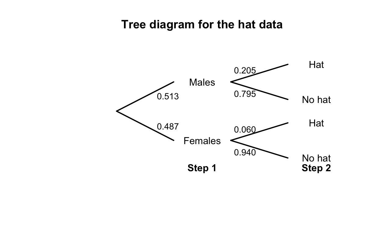
FIGURE F.1: Tree diagram for the hat-wearing example.

TABLE F.1: The numbers of males and females wearing a hat in the middle of the day in Brisbane.
	No Hat	Hat	Total
Males	307	79	386
Females	344	22	366

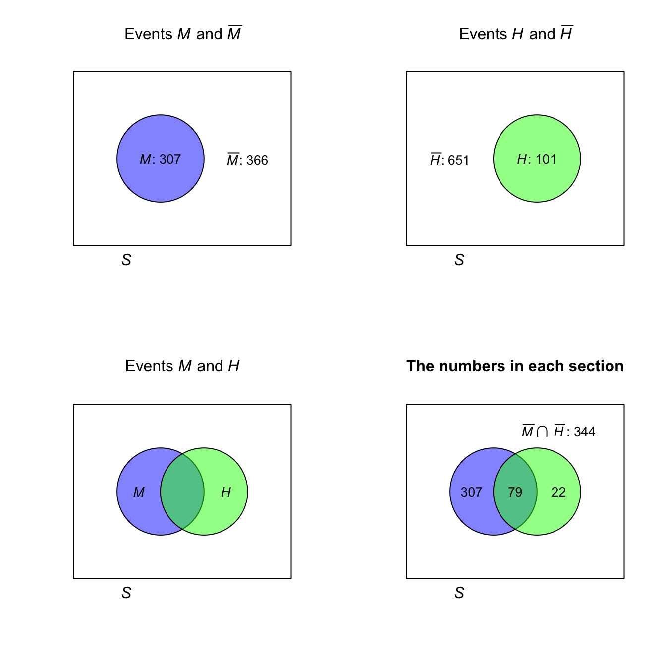
FIGURE F.2: The hat-wearing data as a Venn diagram.

Exercise 3.10.

Choose one driver, and the other seven passengers can sit anywhere: $2!\times 7! = 10\,080$.
Choose one driver, and the other seven passengers can sit anywhere: $3!\times 7! = 30\,240$.
Choose one driver, choose who sits in what car seats, and the other five passengers can sit anywhere: $2!\times 2! \times 5! = 480$.

Exercise 3.11. $8\times 7\times 6\times 5 = 1680$ ways.

Exercise 3.12. The order is important; use permutations.

Eight: $^{26}P_8 = 62\,990\,928\,000$; nine: $^{26}P_9 = 1.133837\times 10^{12}$; ten: $^{26}P_8 = 1.927522\times 10^{13}$. Total: $2.047205\times 10^{13}$.
$^{52}P_8 = 3.034234\times 10^{13}$.
$^{62}P_8 = 1.363259\times 10^{14}$.
TBA.

Exercise 3.13. See Fig. F.3.

# Define a function to compute Stirling numbers:
stirling <- function(n){ 
  sqrt(2 * pi *n) * (n/exp(1))^n
}

n <- 1:10
Actual <- factorial(n) 
Approx <- stirling(n)
RelError <- (Actual - Approx)/Actual * 100

cbind(Actual, Approx, RelError)
#>        Actual       Approx  RelError
#>  [1,]       1 9.221370e-01 7.7862991
#>  [2,]       2 1.919004e+00 4.0497824
#>  [3,]       6 5.836210e+00 2.7298401
#>  [4,]      24 2.350618e+01 2.0576036
#>  [5,]     120 1.180192e+02 1.6506934
#>  [6,]     720 7.100782e+02 1.3780299
#>  [7,]    5040 4.980396e+03 1.1826224
#>  [8,]   40320 3.990240e+04 1.0357256
#>  [9,]  362880 3.595369e+05 0.9212762
#> [10,] 3628800 3.598696e+06 0.8295960

plot(RelError ~ n,
     ylim = c(0, 8),
     las = 1, type = "b",
     pch = 19, lwd = 3,
     xlab = expression(italic(n)),
     ylab = "Relative error (%)",
     main = "Relative error of\nStirling's approximation")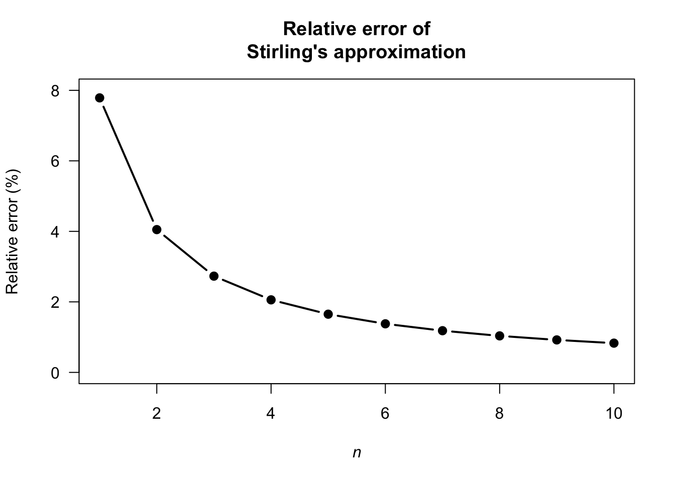

FIGURE F.3: Relative error of Stirling’s approximation.

Exercise 3.14.

()() and (()). There are two ways.
()()() and (())() and ()(()) and ((())) and (()()). There are five ways.
$\displaystyle \frac{1}{n + 1} \binom{2n}{n} = \frac{1}{n + 1}\frac{(2n)!}{n!n!} = \frac{1}{(n + 1)!} \frac{(2n)!}{n!}$ as to be shown.
Write as $\displaystyle \frac{(2n)!}{n!\, n!} - \frac{(2n)!}{(n + 1)! (2n - n - 1)!}$. Simplifying: \[\begin{align*} &\frac{(2n)!}{n!\, n!} - \frac{(2n)!}{(n + 1)! (n - 1)!} = &\frac{(2n)!}{n!\, n!} - \left( \frac{n}{n + 1}\right) \frac{(2n)!}{n!\,n!}\\ = &\binom{2n}{n}\left(1 - \frac{n}{n + 1}\right) \\ = &\frac{1}{n + 1} \binom{2n}{n} \end{align*}\]
The first nine Catalan numbers, for $n = 0, \dots 8$, are $1, 1, 2, 5, 14, 42, 132, 429, 1430$

Exercise 3.15.

$\Pr(\text{Player throwing first wins})$ means $\Pr(\text{First six on throw 1 or 3 or 5 or ...})$. So: $\Pr(\text{First six on throw 1}) + \Pr(\text{First six on throw 3}) + \cdots$. This produces a geometric progression that can be summed obtained (see App. B).
Use Theorem 3.3. Define the events $A = \text{Player 1 wins}$, $B_1 = \text{Player 1 throws first}$, and $B_2 = \text{Player 1 throws second}$.

Exercise 3.16. Write $y = \Pr(\text{answers `yes'})$.

See Fig. F.4.
From Fig. F.4: \[\begin{align*} y &= \Pr(\text{Never takes drugs, and says so}) + \Pr(\text{Takes drugs, and says so})\\ &= (1 - p) \times\left(\frac{N - m}{N}\right) + p\times\frac{m}{N}. \end{align*}\] Solving for the unknown $p$: \[ p = \frac{yN - N + m}{2m - N}. \]
When $m = 0$, $\Pr(Y) = p$: This mean every card says ‘I have used an illegal drug in the past twelve months’, so the proportion that have used an illegal drug is just the same as the proportion responding with ‘Yes’ (and there is no anonymity). When $m = 0$, $\Pr(Y) = 1 - p$: This mean every card says ‘I have not used an illegal drug in the past twelve months’, so the proportion that have used an illegal drug is just the same as the proportion responding with ‘No’ (and there is no anonymity). When $m = N/2$, $\Pr(Y) = 0.5$; we have learnt nothing: The probability is 50–50.
$\displaystyle d = \frac{yN - N + m}{2m - N}$, so plugging in $N = 100$, $m = 25$ and $\Pr(Y) = 175/400 = 0.4375$ gives $d = 0.625$.

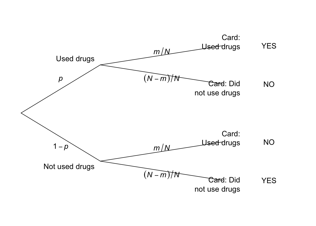
FIGURE F.4: The tree diagram.

Exercise 3.17. Use Theorem 3.3 to find $\Pr(C)$ where $C = \text{select correct answer}$, $K = \text{student knows answer}$. Then, $\Pr(C) = (mp + q)/m$.

Exercise 3.18.

$\Pr(W)$ means ‘the probability of a win’. $\Pr(W \mid D^c)$ means ‘the probability of a win, given the game was not a draw’.
$\Pr(W) = 91/208 = 0.4375$. $\Pr(W\mid D^c) = 91/(208 - 50) = 0.5759494$.

Exercise 3.19. Write $d$ as the distance; then $S = \{d: 0 \le d \le \sqrt{2}\}$. For the grid, let’s use R to find what values are possible:

x <- y <- seq(0, 1, by = 0.25)

distances <- outer(x, y, function(x, y){sqrt(x^2 + y^2)})

unique(sort(distances))
#>  [1] 0.0000000 0.2500000 0.3535534 0.5000000 0.5590170 0.7071068
#>  [7] 0.7500000 0.7905694 0.9013878 1.0000000 1.0307764 1.0606602
#> [13] 1.1180340 1.2500000 1.4142136

There are 15 possible values for the distance:

$0$, $0.25$, $0.50$, $0.75$ and $1$ along grid lines;
$\sqrt{2}/4$, $\sqrt{5}/4$, $\sqrt{10}/4$ and $\sqrt{17}/4$ when the line is moved one grid-square right;
$\sqrt{13}/4$ and $\sqrt{20}/4$ when the line is moved two grid-squares right;
$\sqrt{25}/4$ when the line is moved three grid-squares right;

and so on.

Exercise 3.20.

Anywhere between $0$% and $8$%.
$0.06/0.30 = 0.20$.
$0.06/0.08 = 0.75$.

Exercise 3.21. The total number of children: $69\,279$. Define $N$ as ‘a first-nations student’, $F$ as ‘a female student’, and $G$ as ‘attends a government school’.

$(2540 + 2734 + 391 + 362) / 69,279 \approx 0.0870$.
$49,067/69,279 \approx 0.708$.
Females: prob FN: $0.107$; Males: prob FN: $0.108$; close to independent.
Females: prob FN: $0.040$; Males: prob FN: $0.035$; close to independent.
Gov: prob FN: $0.107$; NGov: prob FN: $0.040$; not independent.
Gov: prob FN: $0.108$; NGov: prob FN: $0.035$; not independent.
Regardless of sex, First Nations children more likely to be at government school.

Exercise 3.22.

The probability depends on what happens with the first card: \[\begin{align*} \Pr(\text{Ace second}) &= \Pr(\text{Ace, then Ace}) + \Pr(\text{Non-Ace, then Ace})\\ &= \left(\frac{4}{52}\times \frac{3}{51}\right) + \left(\frac{48}{52}\times \frac{4}{51}\right) \\ &= \frac{204}{52\times 51} \approx 0.07843. \end{align*}\] You can use a tree diagram, for example.
Be careful: \[\begin{align*} &\Pr(\text{1st card lower rank than second card})\\ &= \Pr(\text{2nd card a K}) \times \Pr(\text{1st card from Q to Ace}) + \qquad \Pr(\text{2nd card a Q}) \times \Pr(\text{1st card from J to Ace}) +{}\\ &\qquad \Pr(\text{2nd card a J}) \times \Pr(\text{1st card from 10 to Ace}) + \dots + \qquad \Pr(\text{2nd card a 2}) \times \Pr(\text{1st card an Ace}) \\ &= \frac{4}{51} \times \frac{12\times 4}{52} + {} \qquad \frac{4}{51} \times \frac{11\times 4}{52} + \qquad \frac{4}{51} \times \frac{10\times 4}{52} + \dots + \qquad \frac{4}{51} \times \frac{1\times 4}{52} s= \frac{4}{51}\frac{4}{52}\left[ 12 + 11 + 10 + \cdots + 1\right]\\ &= \frac{4}{51}\frac{4}{52} \frac{13\times 12}{2} \approx 0.4705882. \end{align*}\]
We can select any of the $52$ cards to begin. Then, there are four cards higher and four lower, so a total of $16 options for the second card, a total of $52\times 16 = 832$ ways it can happen. The number of ways of getting two cards is $52\times 51 = 2652$, so the probability is $832/2652 \approx 0.3137$.

Exercise 3.23. TBA.

Exercise 3.24. $x = 0.05$.

Exercise 3.26. \[\begin{align*} 12\times {}^7P_k &= 7\times {}^6P_{k + 1} \\ 12\times \frac{7!}{(7 - k)!} &= 7\times\frac{6!}{(5 - k)!}\\ \frac{12}{(7 - k)!} &= \frac{1}{(5 - k)!}\\ \frac{12}{(7 - k)\times (6 - k)\times (5 - k)!} &= \frac{1}{(5 - k)!}\\ 12 &= (7 - k)(6 - k)\\ k^2 - 13k + 30 &= 0\\ (k - 10)(k - 3) &= 0 \end{align*}\] and so $k = 10$ or $k = 3$. But if $k = 10$, we get silly things like $P^7_{10}$; the solution must be $k = 3$.

for (k in (1:5)){ # Answer must e less than 6
  cat("FOR k = ", k, ":")
  cat("LHS =", 12 * factorial(7) / factorial(7 - k), "; ")
  cat("RHS =", 7 * factorial(6) / factorial(5 - k), "\n")
}
#> FOR k =  1 :LHS = 84 ; RHS = 210 
#> FOR k =  2 :LHS = 504 ; RHS = 840 
#> FOR k =  3 :LHS = 2520 ; RHS = 2520 
#> FOR k =  4 :LHS = 10080 ; RHS = 5040 
#> FOR k =  5 :LHS = 30240 ; RHS = 5040

Exercise 3.27. \[\begin{align*} \frac{ {}^7 P_{r + 1}}{ {}^{7}C_r} &= \frac{7!}{(7 - (r + 1))!} \times \frac{(7 - r)!\, r!}{7!}\\ &= \frac{7!}{(6 - r)!} \times \frac{(7 - r)!\, r!}{7!}\\ &= \frac{(7 - r)!\, r!}{(6 - r)!}\\ &= \frac{(7 - r)\times (6 - r)!\, r!}{(6 - r)!}\\ &= (7 - r) r!\\ &= 10. \end{align*}\] Rewrite: $r! = 10/(7 - r)$. Since $r!$ is a positive integer, $r$ must be either $r = 2$ or $r = 5$. Trying both, clearly $r = 2$.

Exercise 3.28.

Proceed: \[\begin{align*} \Pr(\text{at least two same birthday}) &= 1 - \Pr(\text{no two birthdays same}) \\ &= 1 - \Pr(\text{every birthday different}) \\ &= 1 - \left(\frac{365}{365}\right) \times \left(\frac{364}{365}\right) \times \left(\frac{363}{365}\right) \times \cdots \times \left(\frac{365 - n + 1}{365}\right)\\ &= 1 - \left(\frac{1}{365}\right)^{n} \times (365\times 364 \times\cdots (365 - n + 1) ) \end{align*}\]
Graph the relationship for various values of $N$ (from $2$ to $60$), using the above form to compute the probability.
No answer (yet).
Birthdays are independent and randomly occur through the year (i.e., each day is equally likely).

N <- 2:80
probs <- array( dim = length(N) )

for (i in 1:length(N)){
  probs[i] <- 1 - prod( (365 - (1:N[i]) + 1)/365 )
}
plot( probs  ~ N,
      type = "l", lwd = 3, las = 1,
      ylab = "Prob. at least two share b'day",
      xlab = expression(Group~size~italic(N)))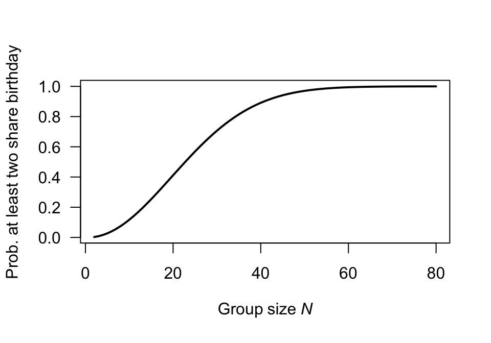

FIGURE F.5: Question 1

Exercise 3.29.

set.seed(981686)
numberSimulations <- 5000
anyConsecutive <- 0

for (i in (1:numberSimulations)){
  # Find the six numbers
  theNumbers <- sample(1:45,
                       size = 6,
                       replace = FALSE)
  theNumbers <- sort(theNumbers)
  
  if (any( diff(theNumbers) == 1 )){
    anyConsecutive <- anyConsecutive + 1
  }
  
}
cat("Number with consecutive values", 
    anyConsecutive,"\n")
#> Number with consecutive values 2691
cat("Proportion with consecutive values", 
    round(anyConsecutive/numberSimulations, 3), "\n")
#> Proportion with consecutive values 0.538
cat("Proportion WITHOUT consecutive values", 
    round(1 - anyConsecutive/numberSimulations, 3), "\n")
#> Proportion WITHOUT consecutive values 0.462

Exercise 3.25. $\Pr( A^c \cap B^c) = 0.5$ (using, for example, a two-way table). $A$ and $B$ are not independent.

Exercise 3.30. $7\times 3\times 2 = 42$.

Exercise 3.31. $10\times 10\times 10\times 26\times 26\times 10 = 6\ 760\ 000$.

Exercise 3.32. Order is not important, so combinations are relevant. There are $\binom{52}{5} = 2\,598\,960$ ways to get five cards from $52$ (without replacement).

Pick the denomination: $13$ to select from. We need two of those $4$ cards: $13\times \binom{4}{2}$. Now the other three cards are drawn from the other $12$ denominations: $\binom{12}{3}$. There are also $4$ ways to choose the suit of each of those $3$ cards. All up then: the number of ways is $13\times\binom{4}{2}\times\binom{12}{3}\times 4^3 = 1\,098\,240$. The probability is therefore $1\,098\,240/2\,598\,960 = 0.422569$. TAKE THE THREE OF A KIND AND FOUR OF A KIND!!
There are $4$ suits each with $4$ picture cards, so $16$ picture cards in total. We want to select five picture cards from $52$ cards, without replacement: $^{16}C_5 = 4\,368$ ways to do this. So the probability is $4\,368\ 160/^{52}C_5 = 0.0017$.

Exercise 3.34. $\binom{25}{8}/\binom{26}{6} = (25!\, 6!\, 19!)/(8!\,17!\,25!) = 171/28 \approx 6.107$.

Exercise 3.35. No answer (yet).

Exercise 3.36. The key: $P$ must lie on a semi-circle with diameter $AB$.

Exercise 3.39.

set.seed(123)

roll_die <- function(die, n) sample(die, n, replace = TRUE)

n <- 1e6
A <- c(2, 2, 4, 4, 9, 9)
B <- c(1, 1, 6, 6, 8, 8)
C <- c(3, 3, 5, 5, 7, 7)

# Simulate rolls
A_rolls <- roll_die(A, n)
B_rolls <- roll_die(B, n)
C_rolls <- roll_die(C, n)

# Compute win probabilities
p_A_beats_B <- mean(A_rolls > B_rolls)
p_B_beats_C <- mean(B_rolls > C_rolls)
p_C_beats_A <- mean(C_rolls > A_rolls)

c(
  "P(A > B)" = p_A_beats_B,
  "P(B > C)" = p_B_beats_C,
  "P(C > A)" = p_C_beats_A
)
#> P(A > B) P(B > C) P(C > A) 
#> 0.555105 0.555608 0.555870

Exercise 3.40. TBA.

Exercise 3.41.

Generate a random sequence of length $1000$ of the digits $1$, $2$ and $3$ to represent which door is hiding the car on each of $1000$ nights.
Generate another such sequence to represent the contestants first choice on each of the $1000$ nights (assumed chosen at random).
The number of times the numbers in the two lists of random numbers do agree represents the number of times the contestant will win if the contestant doesn’t change doors. If the numbers in the two columns don’t agree then the contestant will win only if the contestant decides to change doors.

Recall that the host selects a door that he or she knows does not contains the car.

Generate a random sequence of length $1000$ of the digits $1$, $2$ and $3$ to represent which door is hiding the car on each of $1000$ nights.
Generate another such sequence to represent the contestants first choice on each of the $1000$ nights (assumed chosen at random).
The host then opens a door not chosen by the contestant, that does not contain the car.
The contestant then select from one of the unopened doors.
The number of times the numbers in the two lists of random numbers do agree represents the number of times the contestant will win if the contestant doesn’t change doors. If the numbers in the two columns don’t agree then the contestant will win only if the contestant decides to change doors.

set.seed(93671)        # For reproducibility
num_Reps <- 1000       # Number of simulations

# Initialize counters
Win_By_Switching <- 0
Win_By_Staying   <- 0

for (i in 1:num_Reps) {

  # Step 1: Randomly place the car
  Car_Door <- sample(1:3, 1)

  # Step 2: CONTESTANT makes an initial choice
  First_Choice <- sample(1:3, size = 1)

  # Step 3: HOST then chooses to open a goat door and show contestant.
  #         Host chooses door *not* picked by contestant, or door *not* hiding car
  Possible_Reveals <- setdiff(1:3, c(First_Choice, Car_Door))

  # So Host may now have one or two options of door to open
  if (length(Possible_Reveals) == 1) {
    # With one option... just take it
    Host_Reveal <- Possible_Reveals
  }
  if (length(Possible_Reveals) == 2) {
    # With two options, select one
    Host_Reveal <- setdiff(1:3, First_Choice)
  }

  # Step 4: CONTESTANT may decide to switch to the other unopened door
  Remaining_Door <- setdiff(1:3, c(First_Choice, Host_Reveal))
  Switch_Choice <- Remaining_Door

  # Step 5: Check win conditions
  if (First_Choice == Car_Door) {
    Win_By_Staying <- Win_By_Staying + 1
  } else {
    if (Switch_Choice == Car_Door) {
       Win_By_Switching <- Win_By_Switching + 1
    }
  }
}

# Results
c(Win_By_Staying, Win_By_Switching) / num_Reps
#> [1] 0.336 0.664

Exercise 3.42. First, set up the scenario:

set.seed(8091) # For reproducibility

num_Reps <- 50000     # Number of replications (i.e., simulated days)
daily_Patients <- 20  # Number of patients per day

Then we create an R function to simulate what happens on a day, for any given no-show probability:

# Create an R function to simulate what happens on a day
simulate_Day <- function(no_Show_Prob = 0.15,  # No-show probability
                         num_Patients = 20,    # Number of patients per day
                         patient_Limit = 15) { # More than this many: clinic late
  
  # Allocate a random number between 0 and 1 to each patient
  patient_Probs <- runif( num_Patients)
  
  # sum()  works, because  TRUE = 1,  and  FALSE = 0
  number_No_Shows <- sum( patient_Probs < no_Show_Prob )

  running_Late <- ( (num_Patients - number_No_Shows) > patient_Limit) 
  # TRUE  means clinic will run late.  FALSE  means clinic will NOT run late
  
  return(running_Late)
}

Then run the simulation for the various no-show probabilities:

# Declare the no-show probabilities to use
no_Show_Probs <- seq(0.0, 0.15, by = 0.01)

# Find the mean of the TRUE and FALSE values returned.
# This works because  R  treats TRUE as 1, FALSE as 0
prob_Day_Is_Late <- numeric(length(no_Show_Probs))  # Empty vector

for (i in (1:length(no_Show_Probs)) ){ # For each probability:
  num_Days_Run_Late <- sum(replicate(num_Reps, 
                                     simulate_Day(no_Show_Probs[i]) ) )
  prob_Day_Is_Late[i] <- num_Days_Run_Late / num_Reps
}

The results then can be printed (and plotted; see Fig. F.6):

round(prob_Day_Is_Late, 4)
#>  [1] 1.0000 1.0000 0.9999 0.9998 0.9989 0.9974 0.9945 0.9891
#>  [9] 0.9821 0.9706 0.9567 0.9385 0.9180 0.8916 0.8595 0.8307

plot(prob_Day_Is_Late ~ no_Show_Probs,
     type = "b",     # Plot "both" lines and points
     las = 1,        # Make axis labels horizontal
     lwd = 2,        # Line width of 2
     xlab = "Probability that a patient is a no-show",
     ylab = "Probability that clinic runs late")

Clearly, the greater the no-show probability, the smaller the chance of running late (as expected).

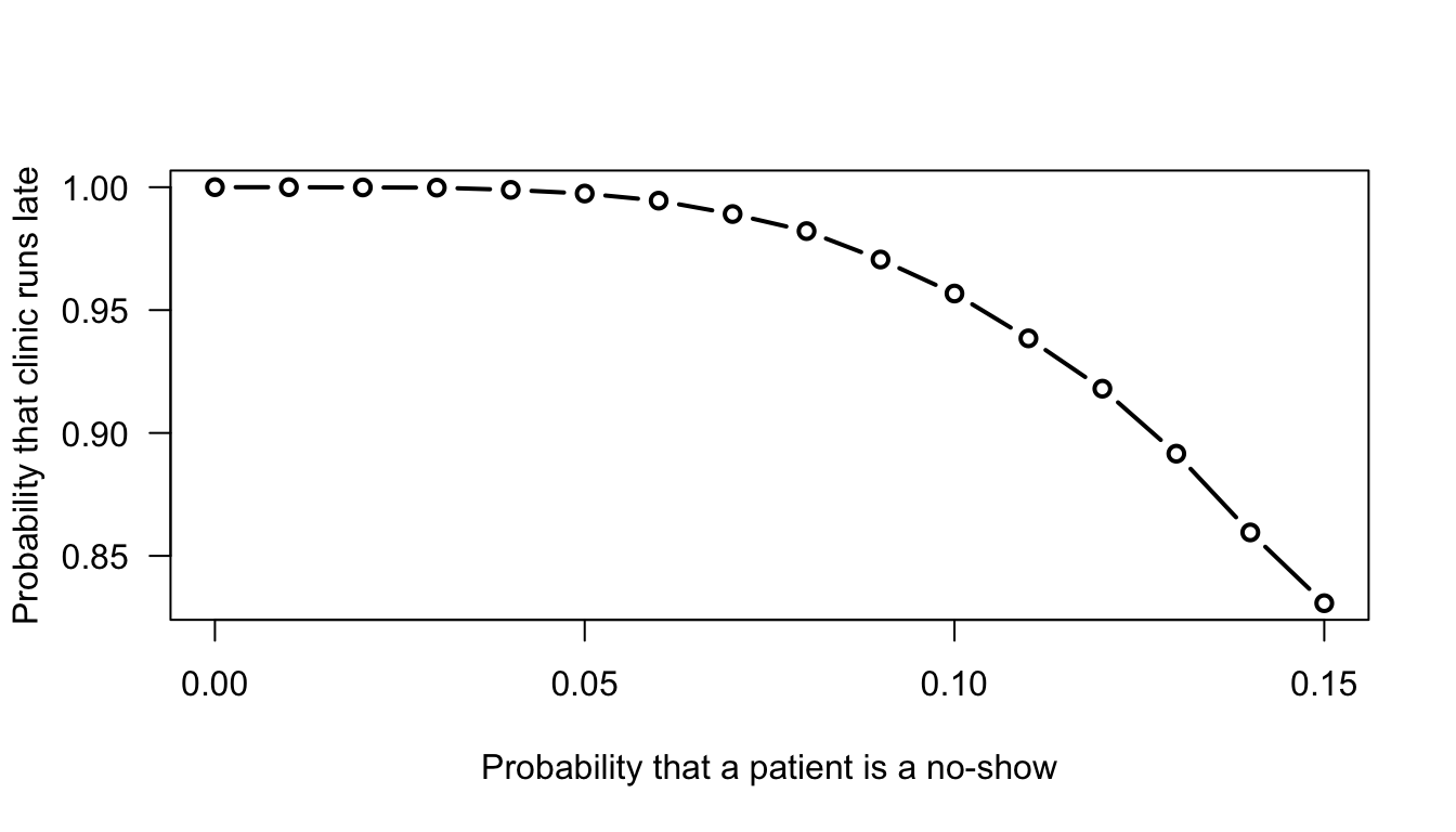
FIGURE F.6: A simulations that shows the probability that a day at a medical clinic runs late.

We could also change the number of patients scheduled each day to see what the impact is (e.g., $18$ or
$25$ patients).

Exercise 3.43.

# 'Make' the deck of cards.
# Note: the denomination is not important, just the suit
Deck <- c(rep("Hearts",   13),   # 13 cards of each suit
          rep("Diamonds", 13), 
          rep("Clubs",    13), 
          rep("Spades",   13))

set.seed(12043)   # For reproducibility 
num_Reps <- 5000  # Number of replications to use

Then we simulate numerous hands of $5$ cards using replicate().

# Each replication goes into a column of  Hands
Hands <- replicate(num_Reps, sample(Deck,               # Sample from the  Deck  
                                    size = 5,           # Hand of *five* cards 
                                    replace = FALSE)  ) # Without replacement
Hands[, 1:4]  # Show the first four columns; each column is a hand of five cards
#>      [,1]       [,2]       [,3]       [,4]    
#> [1,] "Clubs"    "Spades"   "Diamonds" "Clubs" 
#> [2,] "Diamonds" "Spades"   "Hearts"   "Hearts"
#> [3,] "Spades"   "Diamonds" "Diamonds" "Spades"
#> [4,] "Hearts"   "Diamonds" "Diamonds" "Hearts"
#> [5,] "Diamonds" "Diamonds" "Clubs"    "Spades"

Then count the number of Hearts in each Hand (i.e., in each column):

# For each Hand (i.e., column), count how many  Hearts
num_Hearts <- colSums(Hands == "Hearts")

# Show the count of Hearts in those first four hands:
num_Hearts[1 : 4]
#> [1] 1 0 1 2

Then determine how many of these Hands have at least three hearts:

# Count how many have *at least 3* hearts
head(num_Hearts >= 3)    # Show the results from the first few simulations
#> [1] FALSE FALSE FALSE FALSE FALSE FALSE
at_Least_3_Hearts <- sum( num_Hearts >= 3 )

Then estimate the probability, and print the result:

# Compute the *probability* of at least three Hearts
prob_At_Least_3_Hearts <- at_Least_3_Hearts / num_Reps

# Print the (rounded) results (where  "\n"  means to start a new line)
cat("The prob. estimate is", 
    round( mean(prob_At_Least_3_Hearts), 
           4), "\n") # Round to four decimal places
#> The prob. estimate is 0.0978

This is close to what we computed using theory. A more precise estimate would be found using a larger number of simulations.

F.3 Answers for Chap. 4

Exercise 4.1.

$R_X = \{X \mid x \in (0, 1, 2) \}$; discrete.
$R_X = \{X \mid x \in (1, 2, 3\dots) \}$; discrete.
$R_X = \{X \mid x \in (0, \infty) \}$; continuous.
$R_X = \{X \mid x \in (0, \infty) \}$; continuous.

Exercise 4.2.

$R_X = \{X \mid x \in (0, 1, 2, \dots) \}$; discrete.
$R_X = \{X \mid x \in (0, 1, 2, \dots) \}$; discrete.
$R_X = \{X \mid x \in (0, \infty) \}$; continuous.
$R_X = \{X \mid x \in [0, \infty) \}$; mixed.

Exercise 4.5.

The sum of all probabilities is one; none are negative: valid.
Fig. F.7, top left panel.
Fig. F.7, top right panel: $\displaystyle F_X(x) = \begin{cases} 0 & \text{for $x < 10$};\\ 0.3 & \text{for $10 \le x < 15$};\\ 0.5 & \text{for $15 \le x < 20$};\\ 1 & \text{for $x \ge 20$}. \end{cases}$
Fig. F.7, bottom left panel: $\displaystyle F_X(x) = \begin{cases} 1 & \text{for $x < 10$};\\ 0.7 & \text{for $10 \le x < 15$};\\ 0.5 & \text{for $15 \le x < 20$};\\ 1 & \text{for $x \ge 20$}. \end{cases}$
$\Pr(X > 13) = 1 - F_X(13) = 0.7$.
$\Pr(X \le 10 \mid X\le 15) = \Pr(X \le 10) / \Pr(X \le 15) = F_X(10)/F_X(15) = 0.3/0.5 = 0.6$.
Fig. F.7, bottom right panel: Fig. F.7, bottom left panel: $\displaystyle F_X(x) = \begin{cases} 10 & \text{for $0 < p \le 0.3$};\\ 15 & \text{for $0.3 < x \le 0.5$};\\ 20 & \text{for $0.5 < x \le 1$}. \end{cases}$

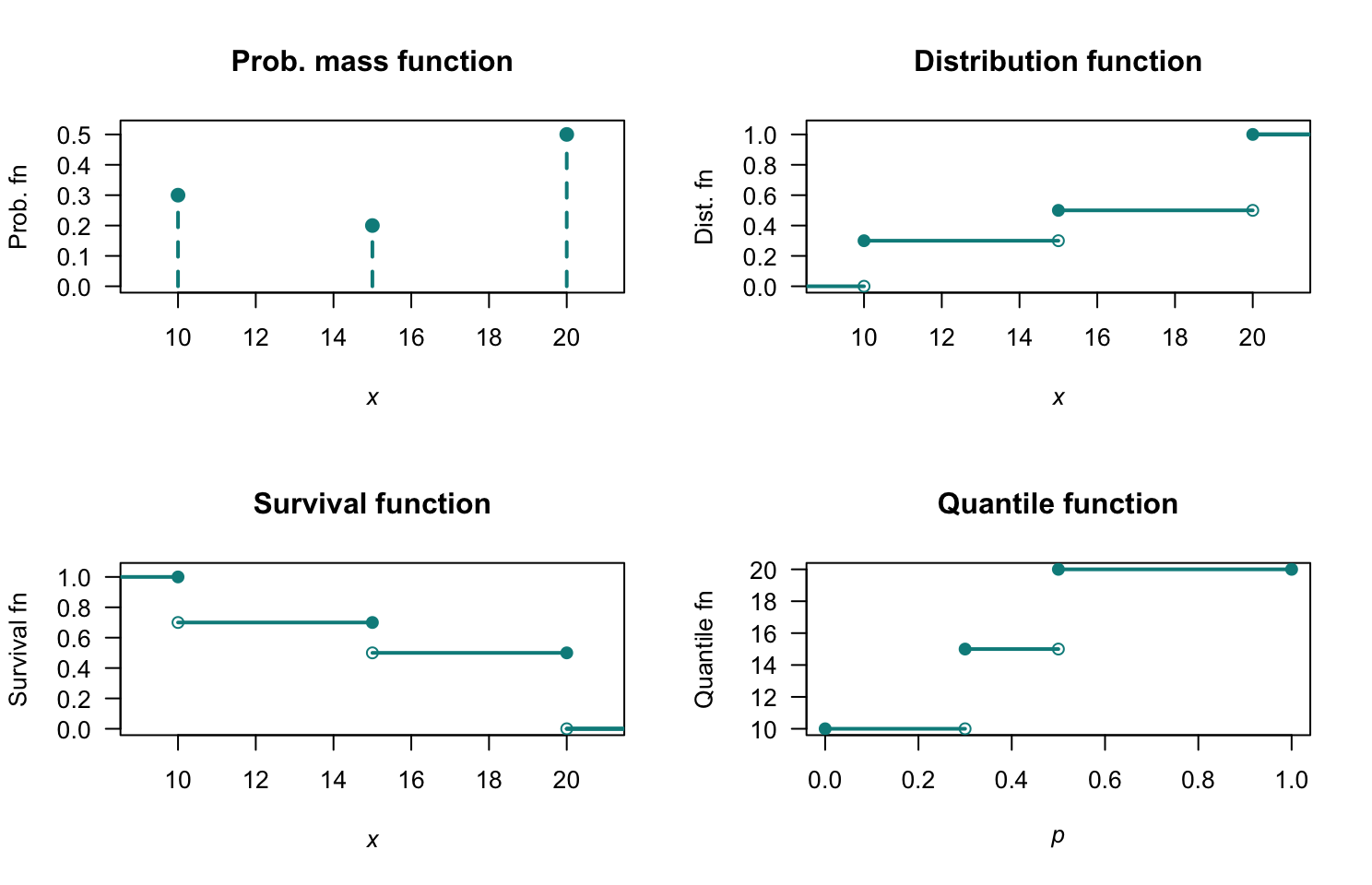
FIGURE F.7: PMF and DF.

Exercise 4.6.

All probabilities are non-negative. Also: $\sum_{x=0}^\infty p_X(x) = \frac{1}{2} + \frac{1}{2}\left(\frac{1}{2}\right) + \frac{1}{2}\left(\frac{1}{2}\right)^2 + \frac{1}{2}\left(\frac{1}{2}\right)^3 + \cdots$. Using Equation (B.5)), with $a = 1/2$ and $r = 1/2$, the sum of this series is $\sum_{x=0}^\infty p_X(x) = 1$. $p_X(s)$ is a valid PDF.
Fig. F.8, top left panel:
Fig. F.8, top right panel. $\displaystyle F_X(x) = \begin{cases} 0 & \text{for $x < 1$};\\ 1 - 2^{-\lfloor x\rfloor} & \text{for $x \ge 1$}. \end{cases}$
Fig. F.8, bottom left panel: $\displaystyle F_X(x) = \begin{cases} 1 & \text{for $x < 1$};\\ 2^{-\lfloor x\rfloor} & \text{for $x \ge 1$}. \end{cases}$
$\Pr(X < 4) = 2^{-1} + 2^{-2} + 2^{-3} = 0.875$.
$\Pr(X\le 2\mid X\le 5) = \Pr(X\le 2)/\Pr(X\le 5) = (3/4)/(31/31) = 24/31 \approx 0.7742$
$Q_X(p) = \lceil -\log_2(1 - p)\rceil$ for $0 < p < 1$. See Fig. F.8, bottom right panel.

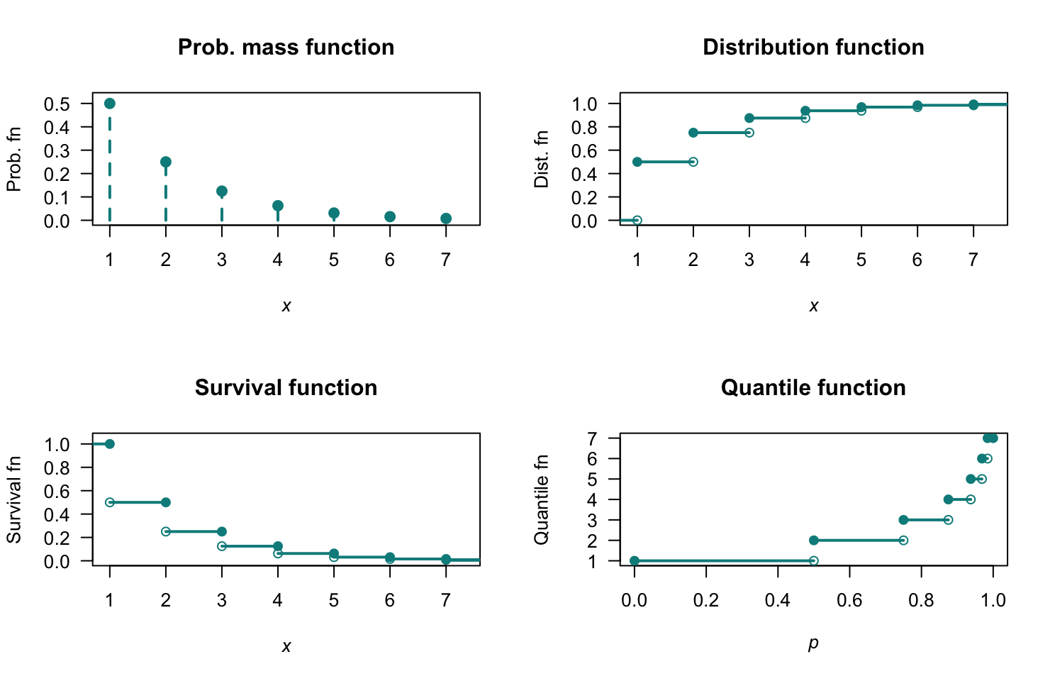
FIGURE F.8: PMF and DF.

Exercise 4.7.

Fig. F.9, top left.
Fig. F.9, top right: $F_X(x) = (x^2 + x - 2)/4$ for $1 < x < 2$.
Fig. F.9, bottom left: $S(x) = 1 - F_X(x)$.
Fig. F.9, bottom right: $Q(p) = (-1 + \sqrt{16p + 9})/2$.

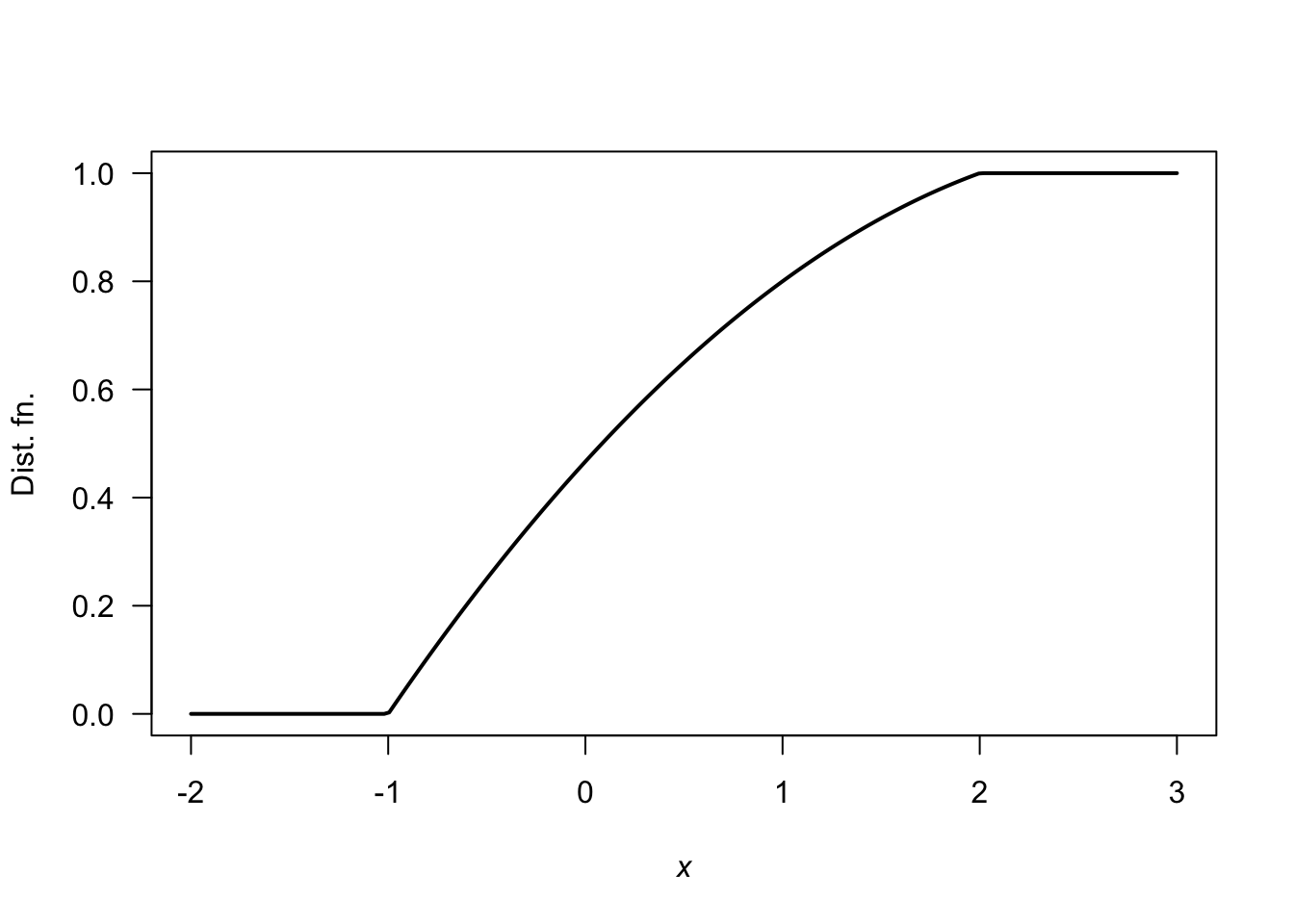
FIGURE F.9: The DF for $X$.

Exercise 4.8.

$\alpha = 2/15$.
Fig. F.10, top left panel.
Fig. F.10, top right panel: $\displaystyle F_Z(z) = \begin{cases} 0 & \text{for $z \le -1$};\\ 6z/15 - z^2/15 + 7/15 & \text{for $-1 < z < 2$};\\ 1 & \text{for $z \ge 2$}. \end{cases}$
Fig. F.10, bottom left panel: $\displaystyle S_Z(z) = \begin{cases} 1 & \text{for $z \le -1$};\\ 81/5 - 6z/15 + z^2/15 & \text{for $-1 < z < 2$};\\ 0 & \text{for $z \ge 2$}. \end{cases}$
$\Pr(Z < 0) = F_Z(0) = 7/15 \approx 0.4666$.
Fig. F.10, bottom right panel: $\displaystyle Q_Z(z) = (6 - \sqrt{64 - 60p})/2$ for $0\le p\le 1$.

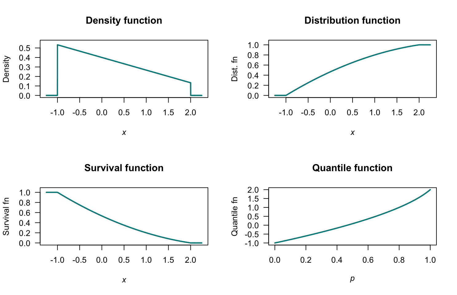
FIGURE F.10: The DF for $Z$.

Exercise 4.9.

Fig. F.11, top left.
Fig. F.11, top right: $F_Y(y) = 0$ for $y < 0$; $F_Y(y) = \sqrt{y+1} - 1$ for $0\le y < 3$; $F_Y(y) = 1$ for $y\ge 3$.
Fig. F.11, bottom left: $S_Y(y) = 1 - F_Y(y) = 2 - \sqrt{y + 1}$ for $0\le y < 3$.
????
Fig. F.11, bottom right: $Q_Y(p) = (1 + p)^2 - 1$ for $0 < p < 1$.
????

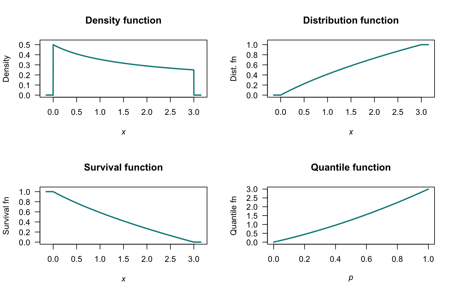
FIGURE F.11: The PDF and DF for $Y$.

Exercise 4.10.

See Fig. F.12 (top left panel).
$F_X(x) = 0$ for $x \le -2$; $F_x(x) = (x^3 +48x + 104)/153$ for $-2 < x < 1$; $F_X(x) = 1$ for $x \ge 1$. See Fig. F.12 (top right panel).
$S_X(x) = 1 - F_X(x)0$. See Fig. F.12 (bottom left panel).
$F_x(3) = 28/63 = 4/9 \approx 0.4444$.
See Fig. F.12 (bottom left panel): $Q_X(p)$ is the unique root of $x^3 + 48x + (104 - 153p) = 0$. $Q_X(0)$: need to solve $x^3 + 48x + 104 = 0$; trying $x = -2$ shows thi sis a root: correct. $Q_X(1)$: need to solve $x^3 + 48x - 49 = 0$; trying $x = 1$ shows this is a root: correct.
Solve $Q_X(0.5)$: $x \approx -0.57$ solving numerically.

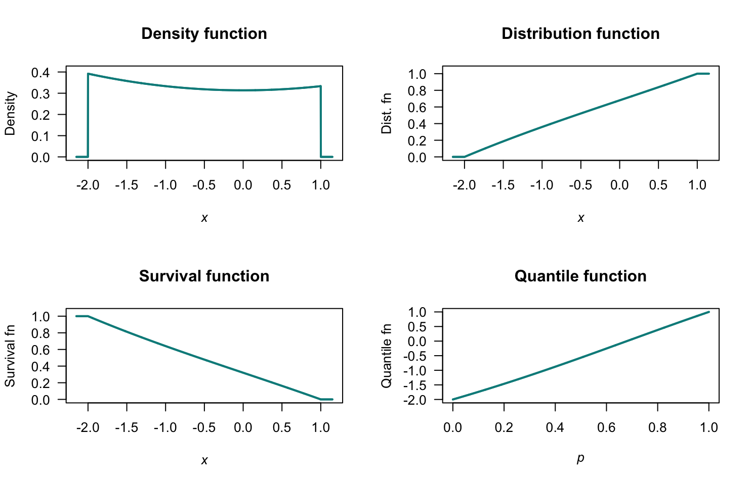
FIGURE F.12: The PDF and DF for $X$.

Exercise 4.11.

$f_T(t) = t + 1\text{\ for $-1 <\le t < 0$}; 1 - t\text{\ for $0\le t \le 1$}$.
$F_T(t) = 0\text{\ for $t < -1$}; (t + 1)^2/2 \text{\ for $-1\le t < 0$}; (1 _ 2t - t^2)/2\text{\ for $0 <\le t < 1$}; 1\text{\ for $t \ge 1$}$.
$S_T(t) = 1 - F_T(t)$.
$Q(p) = 2\sqrt{p} - 1\text{\ for $0 \le p < 1$}; 1 - \sqrt{2 - 2p}\text{\ for $0.5\le p \le 1$}$.

Exercise 4.12.

$a = 2/3$ so $f_Z(z) = 2(1 - z)/3\text{\ for $0 <\le z < 1$}; (z - 2)/3\text{\ for $2\le z \le 4$}$.
$F_Z(z) = 0\text{\ for $z < 0$}; 1/3\text{\ for $1<z<2$}; (2z - z^2)/3 \text{\ for $2\le z < 4$}; 1\text{\ for $t \ge 4$}$.
$S_T(t) = 1 - F_T(t)$.
$Q(p) = 1 - \sqrt{1 - 3p}\text{\ for $0 \le p < 1/3$}; 1/3\text{\ for $1\le p \le 2$}; 2 + \sqrt{6p - 2}\text{\ for $1/3\le p \le 1$}$.

Exercise 4.15.

$F_X(x) = 1 -cos(x)$ for $-\infty < x < \infty$.
$S_X(x) = \cos(x)$ for $-\infty<x<\infty$.
$Q_X(p) = \arccos(1 - p)$ for $0 < p < 1$.

Exercise 4.16.

$F_Y(y) = \exp(y)/2 \text{for $y \le 0$}; 1 - \exp(-t)/2 \text{for $y > 0$}$.
$S_Y(y) = 1 - \exp(y)/2 \text{for $y \le 0$}; \exp(-t)/2 \text{for $y > 0$}$.
$Q_Y(p) = \log(2p) \text{for $0 < p \le 1/2$}; -\log(2(1 - p)) \text{for $<1/2> < p < 1$}$.

Exercise 4.17.

$p = 0.5$.
See below.
For $y < 0$, $F_Y(y) = 0$; for $y = 0$, $F_Y(y) = 0.5$; for $0 < y < 1$, $F_Y(y) = (1 - y^2 + 2y)/2$; for $y \ge 1$, $F_Y(y) = 1$.
$1/8$.

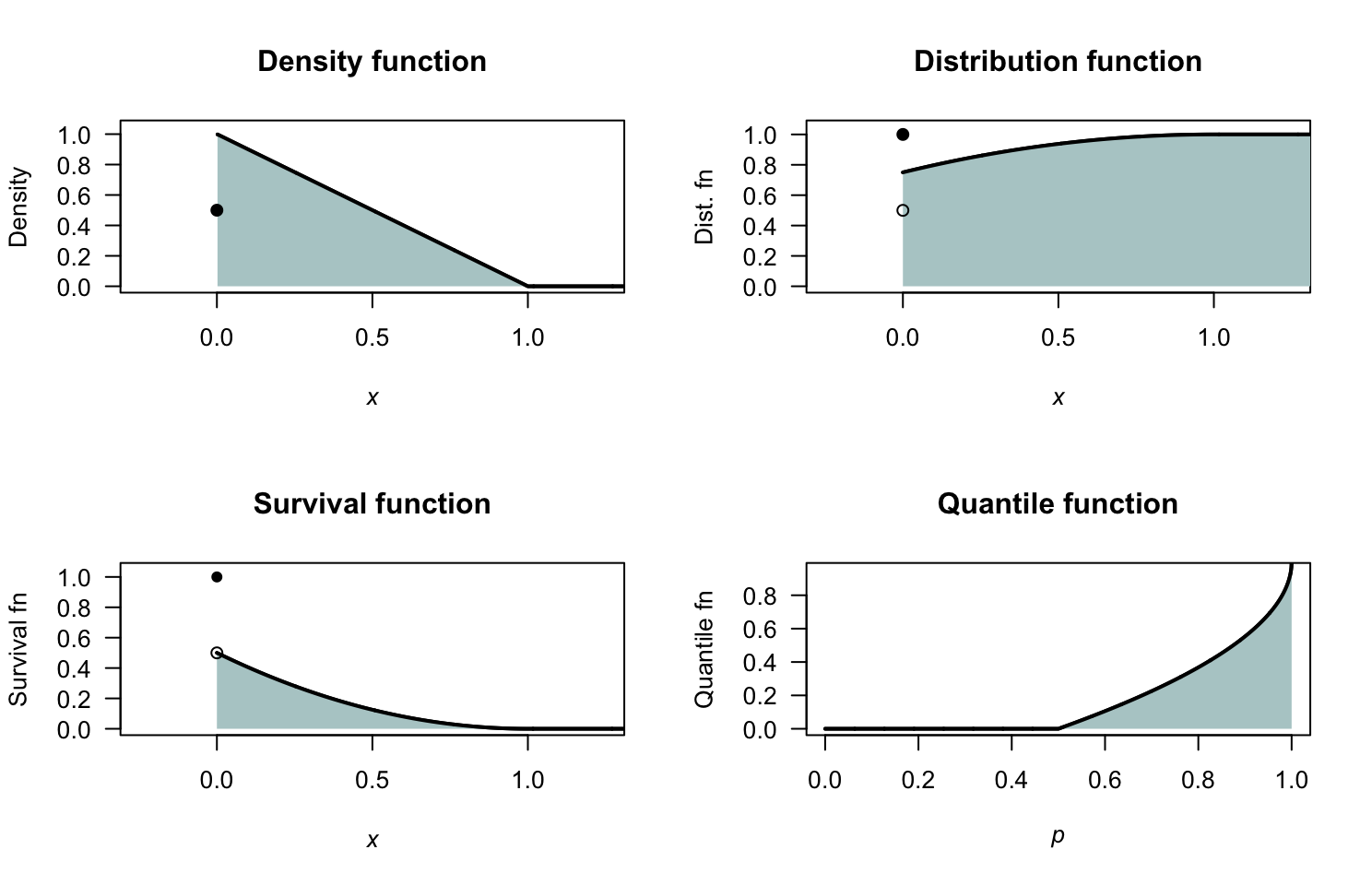
FIGURE F.13: The random variable $Y$.

Exercise 4.18.

$c = 0.25$.
See below.
For $x < 0$, $F_X(x) = 0$; for $x = 0$, $F_X(x) = 0.25$; for $0 < x \ge 1$, $F_X(x) = (1 + x^2)/4$; for $1 < x \ge 3$, $F_X(x) = (6x - 1 - x^2)/8$; for $x > 3$, $F_X(x) = 1$.
$1/2$.

Exercise 4.19.

$a = \sqrt{3} - 1$.

Exercise 4.20.

$c = 3/5$.

Exercise 4.21. $2^\alpha + 4^\alpha = 1$; let $x = 2^a$ leading to $x^2 + x - 1= 0$ and hence $x = 2^a = (\sqrt{5} - 1)/2$ and $a = \log_2[\sqrt{5} - 1 / 2)]\approx -0.694$.

Exercise 4.22. Solving for the mass function to give a total area of one gives $b = -2$. But this produces a negative probability for $x = -2$, so there is no value for $b$ which produces a valid probability function.

Exercise 4.3. $a = 2/3$.

Exercise 4.4. $a = 2/\sqrt{2 + \pi}\approx 0.8820$.

Exercise 4.23.

$\displaystyle p_W(w) = \begin{cases} 0.3 & \text{for $w = 10$};\\ 0.4 & \text{for $w = 20$};\\ 0.2 & \text{for $w = 30$};\\ 0.1 & \text{for $w = 40$}. \end{cases}$
$\Pr(W < 25) = 0.7$.

Exercise 4.24.

$f_Y(y) = (4/3) - y^2$ for $0 < y < 1$.
$\Pr(Y < 0.5) = 0.625$.

fy <- function(y){
  PDFy <- array(0, dim = length(y))
  PDFy <- ifelse( (y > 0) & (y < 1),
                  (4/3) - y^2,
                  0)
  PDFy
}
plotContinuous(pdf_fn = fy,
               type = "PDF",
               lwd = 3,
               col = ColourLight,
               showx = c(-0.25, 1.25) )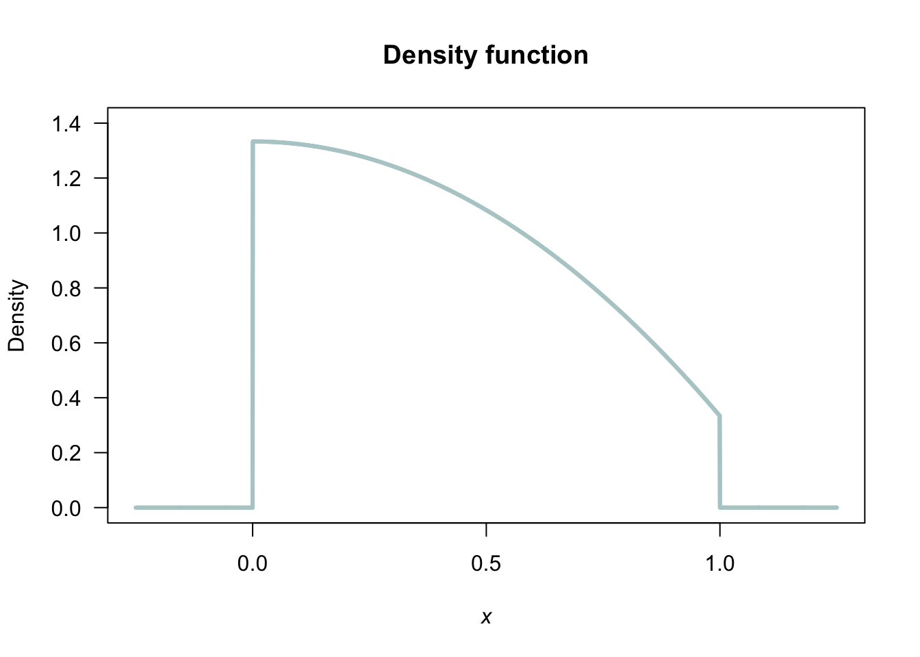

FIGURE F.14: A PDF.

Exercise 4.25.

Easiest to draw, and see that this represents a triangular distribution, and find the area of the said triangle. Integration can be used though.
PDF: \[\begin{align*} f_X(x) &= \begin{cases} \frac{2}{8.8\times 4.4} (x - 0.6) & \text{for $0.6 < x < 5$};\\ \frac{2}{8.8\times 4.4} (9.4 - x) & \text{for $5 < x < 9.4$} \end{cases}\\ &= \begin{cases} \frac{2}{38.72} (x - 0.6) & \text{for $0.6 < x < 5$};\\ \frac{2}{38.72} (9.4 - x) & \text{for $5 < x < 9.4$}. \end{cases} \end{align*}\]
Proceed: \[\begin{align*} F_X(x) &= \begin{cases} 0 & \text{for $x < 0.6$}\\ \int_{0.6}^x \frac{2}{38.72} (t - 0.6) \, dt & \text{for $0.6 \le x < 5$};\\ \int_5^x \frac{2}{38.72} (9.4 - t)\, dt + 0.5 & \text{for $5 \le x < 9.4$}.\\ 1 & \text{for $x \ge 9.4$} \end{cases}\\ &= \begin{cases} 0 & \text{for $x < 0.6$}\\ [(0.6 - x)^2 ]/ 38.72 & \text{for $0.6 \le x < 5$};\\ 1 - [(x - 9.4)^2] / 38.72 & \text{for $5 \le x < 9.4$}.\\ 1 & \text{for $x \ge 9.4$} \end{cases} \end{align*}\]
See below.
$\Pr(X > 3) = 1 - \Pr(X < 3) = 1 - 0.1487603 = 0.8512397$ (or use areas of triangles)
$\Pr(X > 3 \mid X > 1) = \Pr(X > 3) / \Pr(X > 1) = 0.8512397 / 0.9958678 = 0.8547718$.
One is just if $X$ exceeds 3; the other if $X$ exceeds 3 if we already know $X$ has exceeded 1.

f <- function(x){
  f <- array( dim = length(x))
  f[x < 0.6] <- 0
  f[x > 9.4] <- 0
  xSmall <- (x >= 0.6) & ( x <= 5)
  xLarge <- (x > 5) & (x <= 9.4)
  f[xSmall] <- 2 / (8.8 * 4.4) * (x[xSmall] - 0.6)
  f[xLarge] <- 2 / (8.8 * 4.4) * (9.4 - x[xLarge] )
  f
}

F <- function(x){
  FF <- array( dim = length(x))

  for (i in (1:length(x))){
    FF[i] <- integrate(f, lower = 0.6, upper = x[i])$value
  }
  FF
}


par(mfrow = c(1, 2))
x <- seq(0, 10,
         length = 200)
plot( f(x) ~ x,
      type = "l", lwd = 3, las = 1,
      main = "PROB fn",
      xlab = expression(italic(x)),
      ylab = "Prob. fn.")



x <- seq(0, 10,
         length = 200)
plot( F(x) ~ x,
      type = "l", lwd = 3, las = 1,
      main = "DIST fn",
      xlab = expression(italic(x)),
      ylab = "Dist fn.")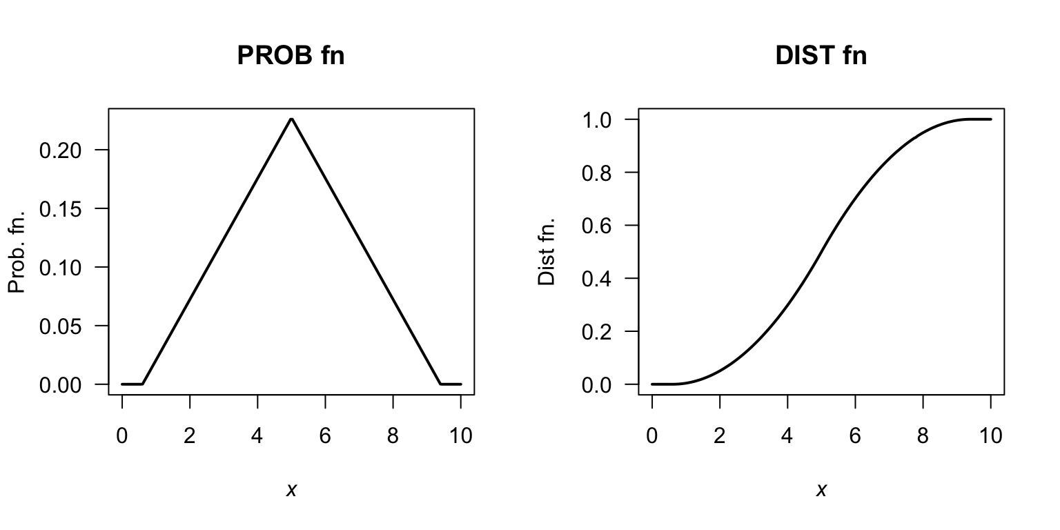

FIGURE F.15: A PDF and DF.

1 - F(3)
#> [1] 0.8512397
(1 - F(3)) / (1 - F(1))
#> [1] 0.8547718

Exercise 4.26. Using the area of triangles, the ‘height’ is $2/27 \approx 0.07407407$ as below. After some algebra: \[ f_S(s) = \begin{cases} \frac{4}{81}s - \frac{14}{81} & \text{for $3.5 < s < 5$};\\ -\frac{4}{1377}s + \frac{122}{1377} & \text{for $5 < s < 30.5$}. \end{cases} \] Also, \[ F_S(s) = \begin{cases} 0 & \text{for $s < 3.5$};\\ \frac{(7 - 2s)^2}{162} & \text{for $3.5 < s < 5$};\\ \frac{2}{1377} (s^2 - 61s + 280) & \text{for $5 < s < 30.5$};\\ 1 & \text{for $s > 30.5$}. \end{cases} \] Then, $\Pr(S > 20 \mid S > 10) = \Pr( (S > 20) \cap (S > 10) )/\Pr(S > 10) = \Pr(S > 20)/\Pr(S > 10) = 0.1601311 / 0.6103854$. This is about $0.2623$.

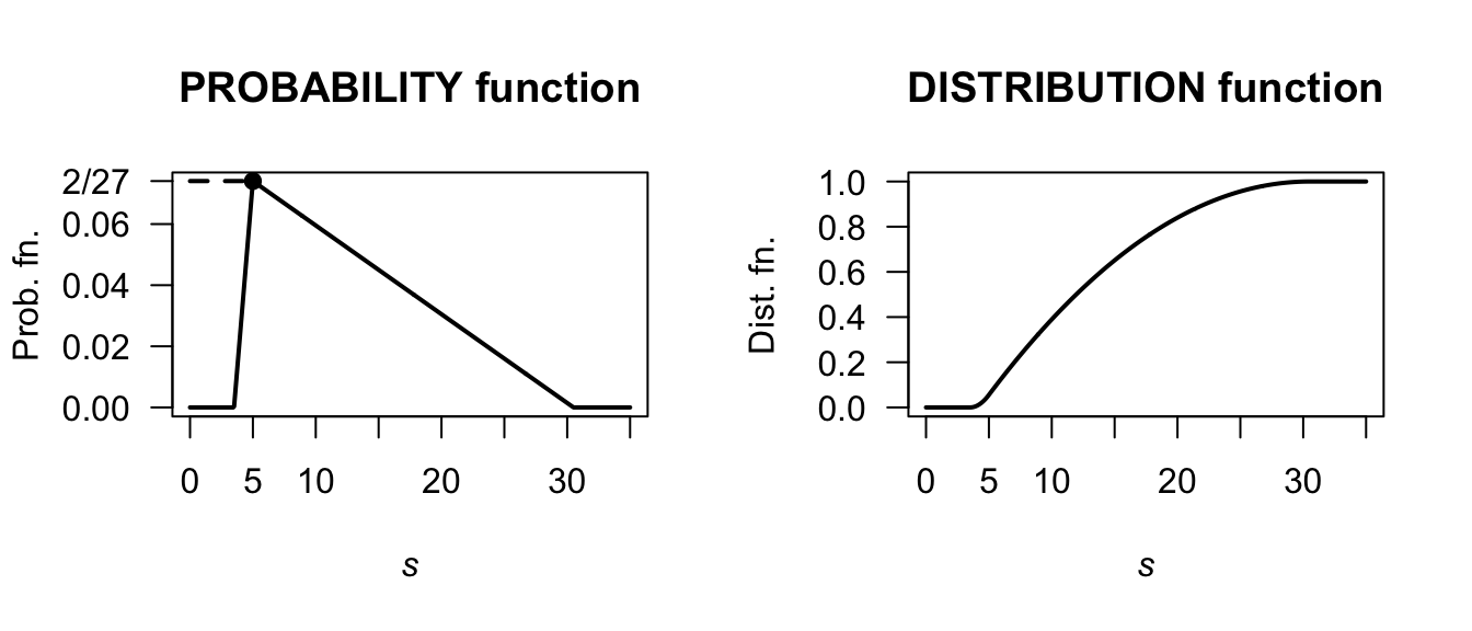
FIGURE F.16: A PDF and DF.

(1 - Fx(20) ) / ( 1 - Fx(10))
#> [1] 0.2623443

Exercise 4.27.

Producers usually need that they will receive at least a certain amount of rainfall.
A very poor graph below; I really have to fix that.
Six months have recorded over $60\,\text{mm}$; so $6/81$. But taking half of the previous ‘40 to under 60’ category, we’d get $12/81$. So somewhere around there.
In June, there are $81$ observations, so the median is the $41st$: The median rainfall is between $0$ to under $20\,\text{mm}$. In December, there are $80$ observations, so the median is the $40.5$th: The median rainfall is between $0$ to under $60\,\text{mm}$.
Median; very skewed to the right.
See below.

#>       Buckets          Jun  Dec 
#>  [1,] "Zero"           "3"  "0" 
#>  [2,] "0 < R < 20"     "41" "17"
#>  [3,] "20 <= R < 40"   "19" "17"
#>  [4,] "40 <= R < 60"   "12" "21"
#>  [5,] "60 <= R < 80"   "2"  "9" 
#>  [6,] "80 <= R < 100"  "2"  "6" 
#>  [7,] "100 <= R < 120" "0"  "3" 
#>  [8,] "120 <= R < 140" "2"  "1" 
#>  [9,] "140 <= R < 160" "0"  "4" 
#> [10,] "160 <= R < 180" "0"  "0" 
#> [11,] "180 <= R < 200" "0"  "1" 
#> [12,] "200 <= R < 220" "0"  "1"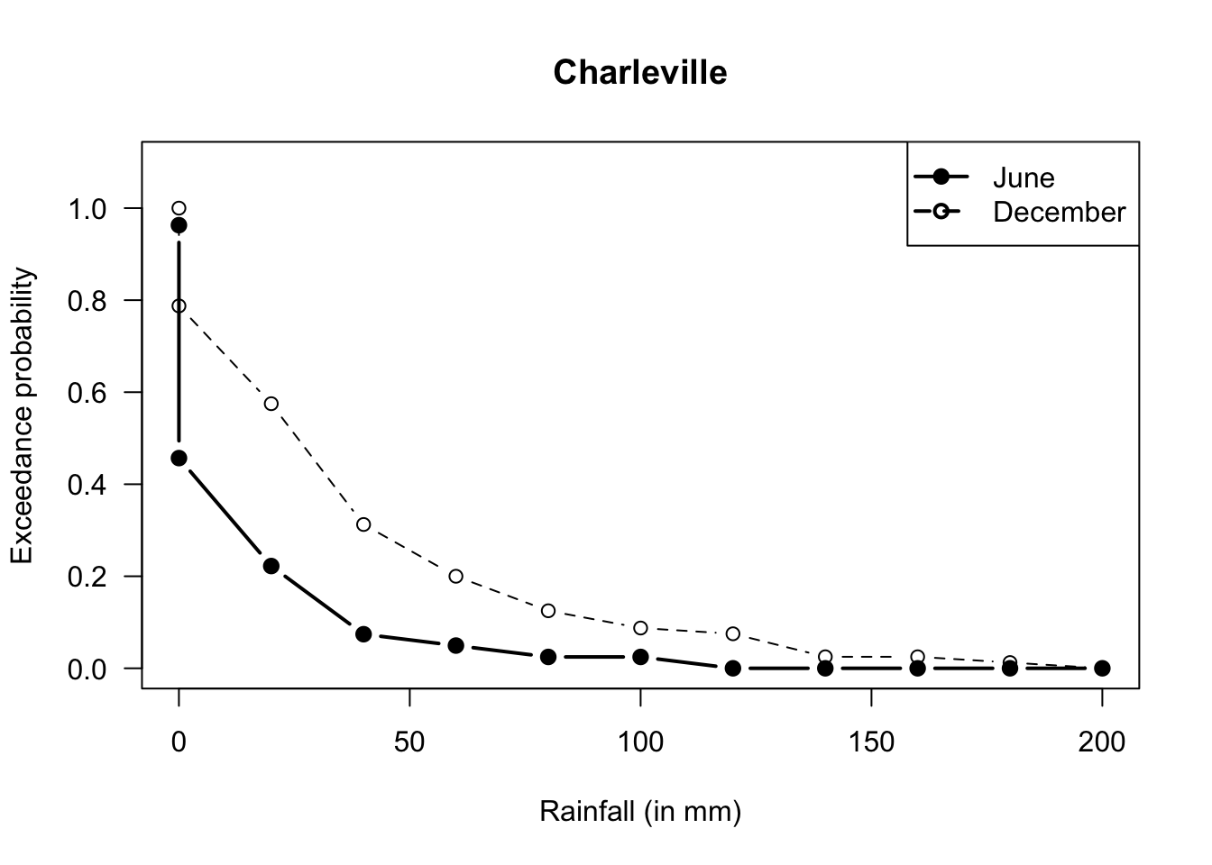

FIGURE F.17: Exceedance charts

Answer for Exercise 4.28. If I stand at Position 1; my friend can be at Positions 2 to 5, with distances $1$, $2$, $3$, $4$. Similar if I stand at Position 5.

If I stand at Position 2; my friend can be at Positions 1, 3 to 5, with distances $1$, $1$, $2$, $3$. Similar if I stand at Position 4.

If I stand at Position 3; my friend can be at Positions 1, 2, 4, 5, with distances $1$, $2$, $2$, $1$.

So counting, the PDF for the number of people between us, say $Y$, is: \[ f_Y(y) = \begin{cases} 4/10 & \text{for $y = 0$};\\ 3/10 & \text{for $y = 1$};\\ 2/10 & \text{for $y = 2$};\\ 1/10 & \text{for $y = 3$}. \end{cases} \] or $f_Y(y) = (4 - y)/10$ for $y\in\{0, 1, 2, 3\}$.

Answer for Exercise 4.13.

$a\int_0^1 (1 - y)^2\,dy = \left[ (1 - y)^3/3\right]_0^1 = 1/3$.
$\Pr(|Y - 1/2| > 1/4) = \Pr(Y > 3/4) + \Pr(Y < 1/4) = 1 - \Pr(1/4 < Y < 3/4) = 13/32$.
See Fig. F.18.

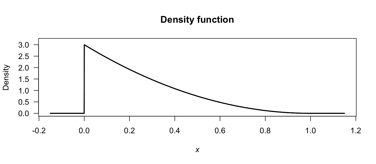
FIGURE F.18: The PDF of $y$.

Answer for Exercise 4.14. df is: \[ F_Y(y) = \begin{cases} 0 & \text{for $y < 0$};\\ \frac{1}{3}(y - 1)^2 & \text{for $1 < y < 2$};\\ \frac{1}{3}(2y - 3) & \text{for $2 < y < 3$};\\ 1 & \text{for $y \ge 3$.} \end{cases} \] When $y = 3$, expect $F_Y(y) = 1$; this is true. When $y = 1$, expect $F_Y(y) = 0$; this is true. For all $y$, $0 \le F_Y(y) \le 1$.

Answer for Exercise 4.30.

See that $X = 1$ (i.e., one pooled test, and all are negative; no further testing needed) or $X = n + 1$ (the pooled test is positive, so $n$ individual tests are needed in addition to the pooled test). The sample space is $\{1, n + 1\}$.
$X = 1$ only occurs if the test is negative; that is, $\Pr(X = 1) = (1 - p)^n$ So: \[ p_X(x) = \begin{cases} (1 - p)^n & \text{for $x = 1$ (i.e., the pooled test is negative)};\\ 1 - (1 - p)^n & \text{for $x = n + 1$ (i.e., individual tests also needed).} \end{cases} \]

Answer for Exercise 4.31. We have cards like: \[ 2, 3, 4, \dots, 8, 9, 10, 10 (J), 10 (Q), 10 (K), 10 (A). \] That is, there are $20$ cards with a points value of ten (four suits of five cards each). For a ‘distance’ say $D$, of $8$, we need $\Pr[ (2, 10)\ \text{or}\ (10, 2)]$, with probability. \[ \Pr(D = 8) = 2\times \left(\frac{4 \times 20}{52 \times 51}\right). \] For a ‘distance’ of $7$, we need \[ \Pr((3, 10)\ \text{or}\ (10, 3)) + \Pr((2, 9)\ \text{or}\ (9, 2)), \] with probability \[ \Pr(D = 7) = 2\times\left(\frac{4 \times 20}{52 \times 51}\right) + 2\times\left(\frac{4 \times 4}{52\times 51}\right). \] For a ‘distance’ of $6$, we need \[ \Pr[(4, 10)\ \text{or}\ (10, 4)] + \Pr[(3, 9)\ \text{or}\ (9, 3)] + \Pr[(2, 8)\ \text{or}\ (8, 2)] \] with probability \[ \Pr(D = 6) = 2\times\left(\frac{4 \times 20}{52 \times 51}\right) + 2\times\left(\frac{4 \times 4}{52\times 51}\right) + 2\times\left(\frac{4 \times 4}{52\times 51}\right). \] So in general, for $D = 1, 2, \dots 8$: \[ \Pr(D = d) = 2\times\left(\frac{4 \times 20}{52 \times 51}\right) + (8 - d)\times 2\times\left(\frac{4 \times 4}{52 \times 51}\right) \]

The case $D = 0$ is different. We can compute the probability as $1$ minus the probabilities from $D = 1$ to $D = 8$, or directly. By subtraction:

d <- 1:8
pd <- (2 * 4 * 20)/(52 * 51) + (8 - d) * (2 * 4 * 4)/(52 * 51)
rbind(d, pd)
#>         [,1]    [,2]      [,3]      [,4]       [,5]       [,6]
#> d  1.0000000 2.00000 3.0000000 4.0000000 5.00000000 6.00000000
#> pd 0.1447964 0.13273 0.1206637 0.1085973 0.09653092 0.08446456
#>          [,7]       [,8]
#> d  7.00000000 8.00000000
#> pd 0.07239819 0.06033183
1 - sum(pd)
#> [1] 0.1794872

To proceed directly, see that a ‘distance’ of zero can occur if we get a ‘ten’ and another ‘ten’, or a non-ten card plus the same non-ten card: \[ \Pr(D = 0) = \frac{20 \times 19}{52 \times 51} + \frac{32\times 3}{52\times 51}. \] The answer is the same:

(20 * 19)/(52 * 51) + (32 * 3)/(52 * 51)
#> [1] 0.1794872

See the PMF in Fig. F.19.

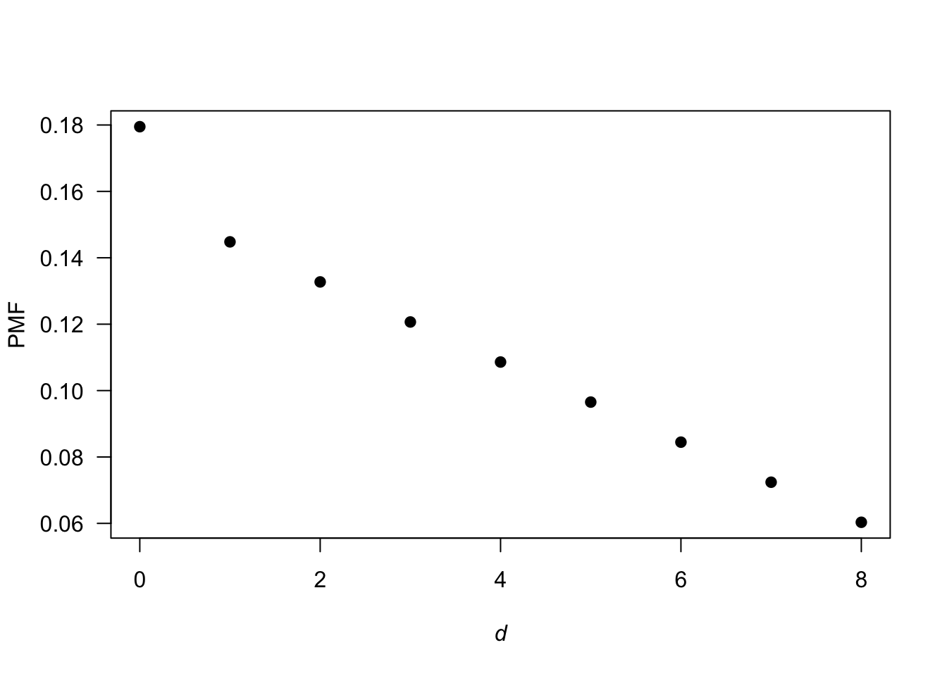
FIGURE F.19: The PDF for the `distance’ between cards.

Answer for Exercise 4.32.

Write as $p(x) = \log_{10}(1 + x) - \log_{10}x$; then the sum is \[\begin{align*} (\log_{10}(2) - \log_{10} 1) + (\log_{10} 3 - \log_{10} 2) + (\log_{10} 4 - \log_{10} 3) + \dots\\ + (\log_{10} 9 - \log_{10} 8) + (\log_{10} 10 - \log_{10} 9) \end{align*}\] and things cancel, leaving $\log_{10}10 = 1$.
The DF is \[\begin{align*} F_D(d) &= \sum_{i = 1}^d \log[ (1 + d)/ \log(d) ] \\ &= \sum_{i = 1}^d \log(1 + d) - \log d\\ &= (\log 2 - \log 1) + (\log 3 - \log 2) + \log 4 - \log 3) + \cdots\\ & \quad {} + (\log d - \log(d - 1) ) + (\log (1 + d) - \log d)\\ &= \log (1 + d). \end{align*}\]

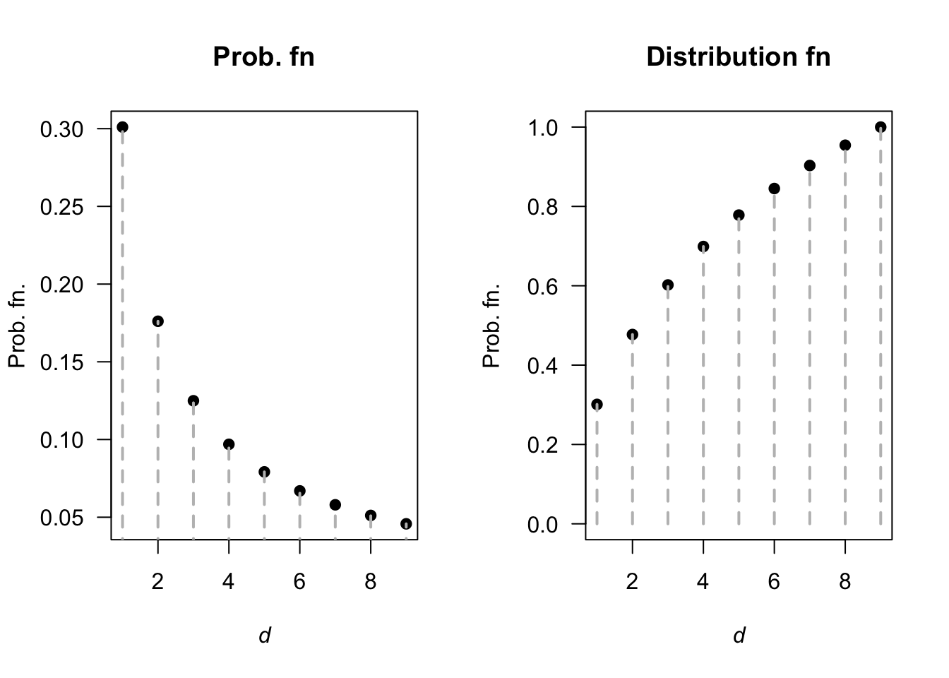
FIGURE F.20: A PDF and DF.

Answer for Exercise 4.33. $k = 1/\pi$. $F(y) = \int_0^x \frac{1}{\pi\sqrt{t(1 - t)}}\, dt = \frac{1}{\pi}\arcsin(2x - 1) + \frac{1}{2}$ for $0 < x < 1$. $\Pr(X > 0.25) = 2/3$.

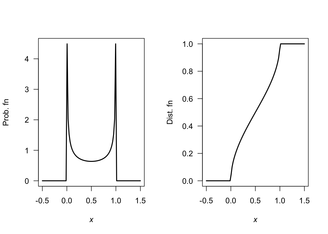
FIGURE F.21: A PDF and DF.

Answer for Exercise 4.34. The PDF is \[ f_X(x) = \frac{d}{dx} \exp(-1/x) = \frac{\exp(-1/x)}{x^2} \] for $x > 0$. See Fig. F.22.

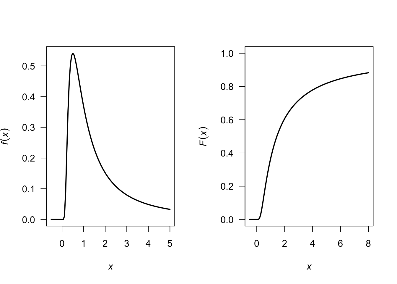
FIGURE F.22: A PDF and DF.

Answer for Exercise 4.29.

1 suit: Select 4 cards from the 13 of that suit, and there are four suits to select.
2 suits: There are two scenarios here:
- Three from one suit, and one from another: Choose a suit, and select three cards from it: $\binom{4}{3}\binom{13}{3}$. Then we need another suit (three choices remain) and one card from (any of the 13).
- Chose two suits, and two cards from each of two suits: $\binom{4}{2}\binom{13}{2}\binom{13}{2}$
3 suits: Umm…
4 suits: Choose one from each of the four suits.

One way to get 3 suits is to realise that the total probability must add to one…

### 1 SUIT
suits1 <- 4 * choose(13, 4) / choose(52, 4)

### 2 SUITS
suits2 <- choose(4, 3) * choose(13, 3) * choose(3, 1) * choose(13, 1) + 
          choose(4, 2) * choose(13, 2) * choose(13, 2)
suits2 <- suits2 / choose(52, 4)

### 4 SUITS:
suits4 <- choose(13, 1) * choose(13, 1) * choose(13, 1) * choose(13, 1)
suits4 <- suits4  / choose(52, 4)

suits3 <- 1 - suits1 - suits2 - suits4

round( c(suits1, suits2, suits3, suits4), 3)
#> [1] 0.011 0.300 0.584 0.105

Answer for Exercise 4.36. I have no idea… From ChatGPT (i.e., haven’t checked) these.

At least four:

# Set the number of simulations
num_simulations <- 100000

# Initialize a vector to store the number of rolls required for each simulation
rolls_required <- numeric(num_simulations)

# Function to simulate rolling a die until the total is 4
simulate_rolls <- function() {
  total <- 0
  rolls <- 0
  while (total < 4) {
    roll <- sample(1:6, 1) # Roll the die
    total <- total + roll
    rolls <- rolls + 1
  }
  return(rolls)
}

# Perform simulations
for (i in 1:num_simulations) {
  rolls_required[i] <- simulate_rolls()
}

# Calculate the PMF
PMF <- table(rolls_required) / num_simulations

# Print the PMF
print(PMF)

# Optionally, plot the PMF
barplot(PMF, main = "Probability Mass Function of Rolls Needed to Sum to 4",
        xlab = "Number of Rolls", ylab="Probability")

Exactly four:

# Set the number of simulations
num_simulations <- 100000

# Initialize a vector to store the number of rolls required for each simulation
rolls_required <- integer(num_simulations)

# Function to simulate rolling a die until the total is exactly 4
simulate_rolls <- function() {
  total <- 0
  rolls <- 0
  while (total < 4) {
    roll <- sample(1:6, 1) # Roll the die
    total <- total + roll
    rolls <- rolls + 1
    if (total > 4) {
      return(NA) # Return NA if the total exceeds 4
    }
  }
  return(rolls)
}

# Perform simulations
for (i in 1:num_simulations) {
  result <- simulate_rolls()
  if (!is.na(result)) {
    rolls_required[i] <- result
  }
}

# Remove NA values from the results
rolls_required <- na.omit(rolls_required)

# Remove zero values (impossible cases)
rolls_required <- rolls_required[rolls_required > 0]

# Calculate the PMF
PMF <- table(rolls_required) / length(rolls_required)

# Print the PMF
print(PMF)

# Optionally, plot the PMF
barplot(PMF, main = "Probability Mass Function of Rolls Needed to Sum to 4",
        xlab = "Number of Rolls", ylab = "Probability")

Answer for Exercise 4.37. 1. $4ab = 1$. 2. $f_X(x) = (x + 16)/32$ for $-1 < x < 1$. 3. $F_X(x) = (x^2 + 32x + 31)/64$ for $-1 < x < 1$. 4. $Q_X(p) = -16 + \sqrt{225 + 64 p}$ for $0 < p < 1$. $Q_X(0) = -1$ as expected; $Q_X(1) = 1$ as expected. 5. See Fig. F.23.

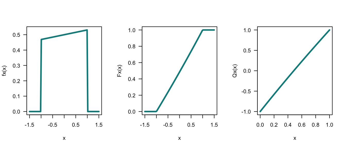
FIGURE F.23: PDF, DF and quantile functions.

F.4 Answers for Chap. 5

Answer for Exercise 5.1.

$k = -2$.
See Fig. F.24 (left panel).
$\operatorname{E}[Y] = 5/3$.
$\operatorname{E}[Y^2] = 17/6$, so $\operatorname{var}[Y] = 17/6 - (5/3)^2 = 1/18$.
$\Pr(X > 1.5) = \int_{1.5}^2 f_Y(y)\, dy = 3/4$.

Answer for Exercise 5.2.

See Fig. F.24 (right panel).
$\operatorname{E}[X] = \int_{-1}^0 2x(x + 1)/3\, dx + \int_{0}^2 x(2 - x)/3\, dx = -\frac{1}{9} + \frac{4}{9} = 1/3$.
$\operatorname{E}[X^2] = (1/18) + (4/9) = 9/18 = 1/2$. So $\operatorname{var}[X] = (1/2) - (1/3)^2 = 7/18\approx 0.38889$.

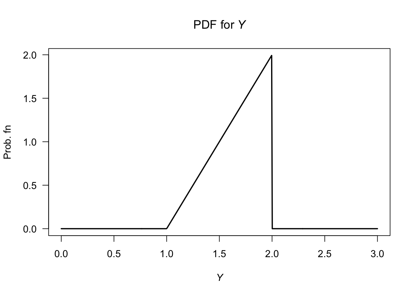
FIGURE F.24: The PDF for $Y$ (left) and for $X$ (right).

Exercise 5.3.

See Fig. F.25 (left panel).
$\operatorname{E}[X] = (1/4) + (2/3) = 11/12$.
$\operatorname{E}[T^2] = (1/6) + (11/12) = 13/12$. So $\operatorname{var}[T] = (13/12) - (11/12)^2 = 35/144\approx 0.2431$.
$F_T(t) = t/2$ for $0 < t < 1$; $F_T(t) = (1/2) - (t - 3)(t - 1)/2$ for $1 < t < 2$. See Fig. F.25 (right panel).
$F_T(t = 1) = 1/2$.

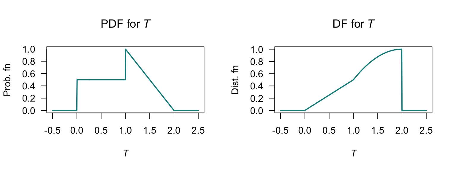
FIGURE F.25: The PDF for $T$ (left) and DF for $T$ (right).

Exercise 5.4.

See Fig. F.26 (left panel).
$\operatorname{E}[Z] = (1/6) + (4/3) = 3/2$ as expected.
$\operatorname{E}[Z^2] = (1/12) + (43/12) = 15/4$. So $\operatorname{var}[Z] = (15/4) - (3/2)^2 = 17/12 \approx 1.416$.
$F_Z(z) = z(1 - z)/2$ for $0 < z < 1$; $F_Z(z) = (z^2 - 4z + 5)/2$ for $2 < z < 3$; See Fig. F.26 (right panel).
$\Pr(Z > 2\mid Z > 1) = \Pr(Z > 2)/\Pr(Z > 1)$. Then, $\Pr(Z > 2) = 1 - F_Z(z = 2) = 1/2$ and $\Pr(Z > 2) = 1 - F_Z(z = 2) = 1/2$. Thus, $\Pr(Z > 2\mid Z > 1) = 1$, which should be obvious from a plot of the PDF.

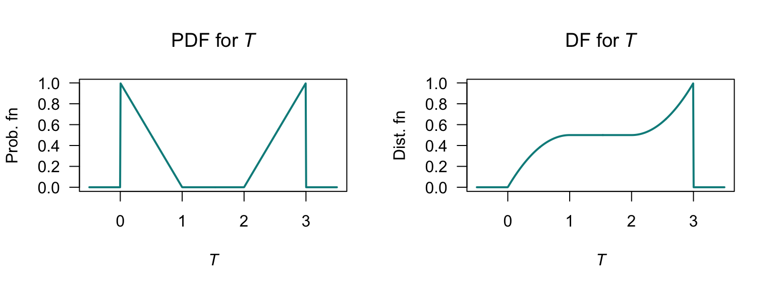
FIGURE F.26: The PDF for $Z$ (left) and the DF for $Z$ (right).

Exercise 5.5. First: $k = 1/4$.

Plot not shown.
$\operatorname{E}[D] = 7/4 = 1.75$; $\operatorname{E}[D^2] = 15/4$ so $\operatorname{var}[D] = 11/16 = 0.6875$.
$M_D(t) = \exp(t)/2 + \exp(2t)/4 + \exp(3t)/4$.
Mean and variance as above.
$\Pr(D < 3) = 3/4$.

Exercise 5.6. First, $c = 144/205$.

See Fig. F.27 (right panel).
$\operatorname{E}[Z] = \frac{144}{205} \sum_{z=1}^4 1/z = 60/41\approx 1.463$. $\operatorname{E}[Z^2] = \frac{576}{205}\approx 2.810$ and so $\operatorname{var}[Z] = (576/205) - (60/41)^2 = 5616/8405\approx 0.6682$.
$M_Z(t) = \frac{\exp(t)}{205}(36\exp(t) + 16\exp(2t) + 9\exp(3t) + 144)$.
Mean and variance as above.
$\Pr(Z \ge 2) = 1 - \Pr(Z = 1) = 61/205$.

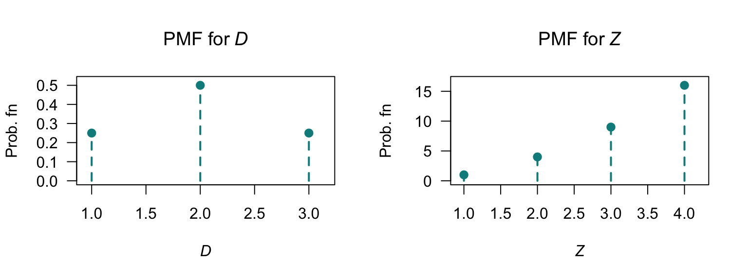
FIGURE F.27: The PMF for $D$ (left) and the PMF for $Z$ (right).

Exercise 5.9.

$M_Z'(t) = 0.6\exp(t)[0.3\exp(t) + 0.7]$ so $\operatorname{E}[Z] = 0.6$. Also, $M''_Z(t) = 0.18\exp(2t) + 0.6\exp(t)[0.3\exp(t) + 0.7]$ so $\operatorname{E}[Z^2] = 0.78$, so $\operatorname{var}[Z] = 0.42$ (be careful with the derivatives here!)
Expand the quadratic and find: $\Pr(Z = 0) = 0.49$, $\Pr(Z = 1) = 0.42$, $\Pr(Z = 2) = 0.09$.

Exercise 5.10.

$\operatorname{E}[W] = (1 - p)/p$; $\operatorname{var}[W] = (1 - p)/p^2$.
$p_W(w) = (1 - p)^w$ for $w = 1, 2, \dots$.

Exercise 10.19.

$17$.
$5 + 2 + (2\times 0.2) = 7.4$.
$14$.
$(2^2\times 5) + ((-3)^2\times 2) + 2\times(2\times -3\times 0.2) = 35.6$.

Exercise 5.14. $[exp(tb) - \exp(ta)]/[t (b - a)]$ for $t\ne 0$.

Exercise 5.11.

$M'_G(t) = \alpha\beta(1 - \beta t)^{-\alpha - 1}$ so $\operatorname{E}[G] = \alpha\beta$. $M''_G(t) = \alpha\beta^2(\alpha + 1)(1 - \beta t)^{-\alpha - 2}$ so $\operatorname{E}[G^2] = \alpha\beta^2(\alpha + 1)$ and $\operatorname{var}[G] = \alpha\beta^2$.

Exercise 5.12.

Proceed: \[ \mu'_r = \operatorname{E}[X^r] = \int_{x = 0}^1 x^r 2(1 - x)\, dx = 2\left[ \left(\frac{x^{r + 1}}{r + 1} - \frac{x^{r + 2}}{r + 2}\right)\right]_{0}^{1} = 2\left[ \frac{1}{r + 1} - \frac{1}{r + 2}\right]. \]
Expanding, $\operatorname{E}[(X + 3)^2] = \operatorname{E}[X^2] + 6\operatorname{E}[X] + 9$. Now, $\operatorname{E}[X] = \mu'_1 = 1/3$ from above, and $\operatorname{E}[X^2] = \mu'_2 = 1/6$ from above. Hence $\operatorname{E}[(X + 3)^2] = 67/6$.
$\operatorname{var}[X] = \operatorname{E}[X^2] - \operatorname{E}[X]^2 = 1/18$.

Exercise 10.18.

$13 + 4 = 17$.
$5 + 2 = 7$.
$(2\times 13) - (3\times 4) = 14$.
$(2^2\times 5) + (-3)^2\times 2) = 38$.

Answer to Exercise 10.19.

$17$.
$7.4$.
$14$.
$35.6$.

Exercise 5.15. $\left[6\left( (t - 2)\exp(t) + t + 2\right)\right]/t^3$ for $t\ne 0$.

Exercise 5.16.

$\operatorname{E}[Y] = \int_2^\infty y\frac{2}{y^2}\,dy = \left[2\log y\right]_2^\infty$, which does not converge.
If $\operatorname{E}[Y]$ is not defined, then $\operatorname{var}[Y]$ cannot be defined either.
See Fig. F.28, left panel.
$F_Y(y) = \int_2^y 2/t^2\, dt = 1 - (2/y)$; see Fig. F.28, right panel.
$F_Y(y) = 0.5$ gives the median as $4$.
$F_Y(y) = 1/4$ gives $Q_1 = 8/3$; $F_Y(y) = 3/4$ gives $Q_3 = 8$; so IQR is $8 - 8/3 = 16/3$.
$\Pr(Y > 4\mid Y > 3) = \Pr(Y > 4)/\Pr(Y > 3)$. Then, $\Pr(Y > 4) = 1 - \Pr(Y < 4) = 1/2$ using the df; and $\Pr(Y > 3) = 1 - \Pr(Y < 3) = 2/3$ using the df; so the answer is $3/4$.

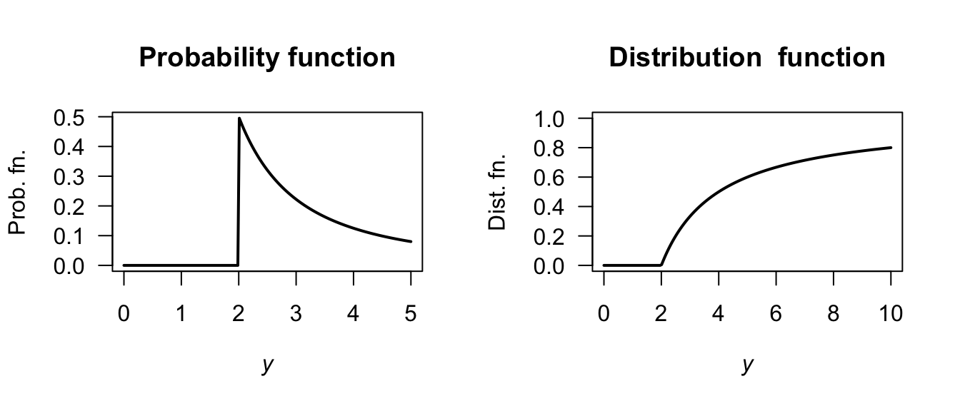
FIGURE F.28: The probability and distribution functions for a distribution with no mean.

Exercise 5.17.

See Fig. F.29 (left panel).
Evaluate $F_X(t) = \displaystyle \int_{-\infty}^t \frac{1}{\pi(1 + x^2)}\,dx = \frac{1}{\pi}\arctan(x) + \frac{1}{2}$. See Fig. F.29 (right panel).
$\displaystyle \operatorname{E}[X] = \int_{-\infty}^t \frac{x}{\pi(1 + x^2)}\,dx = ...$, which is not defined.

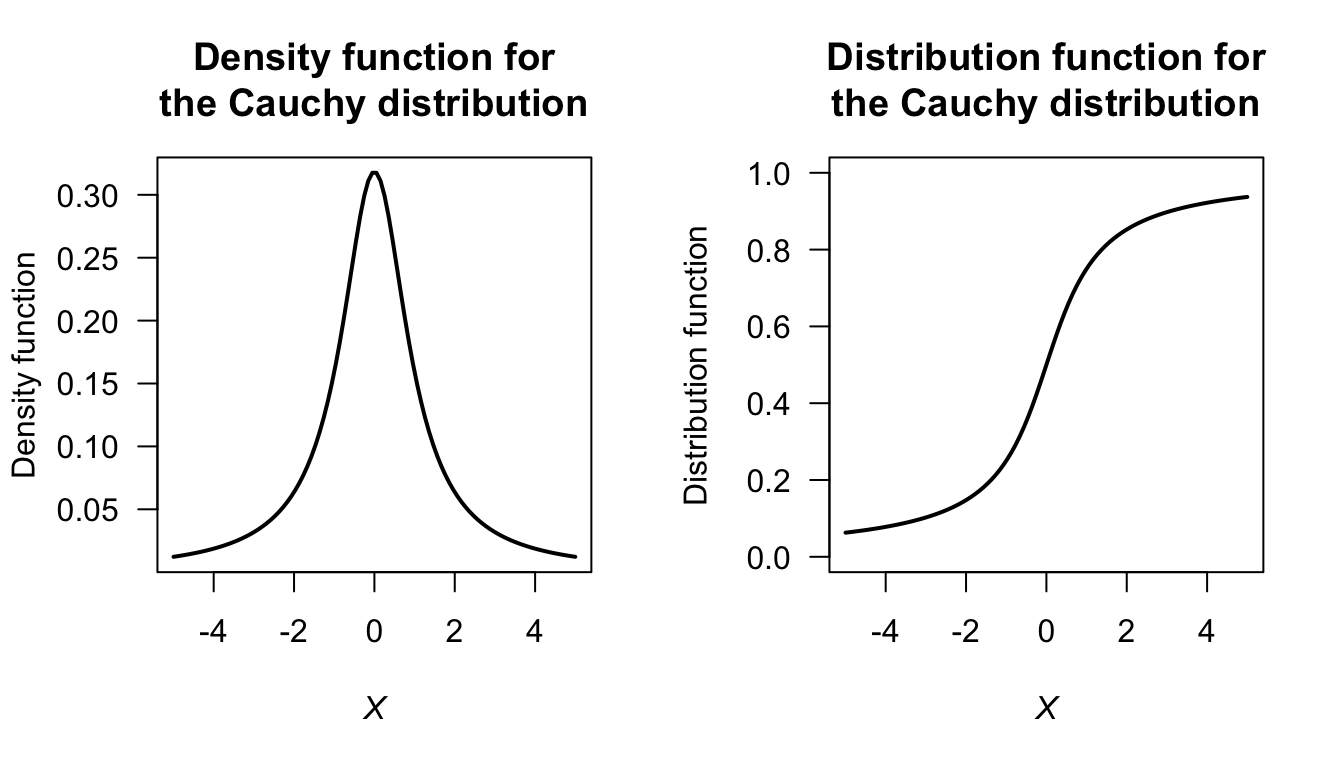
FIGURE F.29: The Cauchy distribution.

Exercise 5.19. Begin with Definition 5.10 for $M_X(t)$ and use fact that if a distribution is symmetric about $0$ then $f_X(x) = f_X(-x)$ using symmetry. Transform the resulting integral.

Exercise 5.20.

Any real $a$ satisfies the integral condition. For non-negativity, need $a \ge -1$ and $a \le -3$.
$\operatorname{E}[X] = (3a + 7)/(3a+6)$, so need $a = -1$: $f_X(x) = x/2$ for $0\le x\le 2$.

Exercise 5.21.

On solving, find $a = 1$ or $a = 1/2$.
For $a = 1$, $\operatorname{E}[X] = 1/2$. For $a = 1/2$, $\operatorname{E}[X] = 31/60 > 1/2$, so $a = 1/2$.

Exercise 5.22. First, the PDF needs to be defined (see Fig. F.30), and define $W$ as the waiting time. Let $H$ be the ‘height’ of the triangle. The area of triangle $A_1$ is $3H/4$, and the area of triangle $A_2$ is $51H/4$, so $H = 2/27$.

The two lines, $L_1$ and $L_2$ can be found (find the slope; determine the linear equation) so that: \[ f_W(w) = \begin{cases} 4w/81 - 14/81 & \text{for $3.5 < w < 5$};\\ -4w/1377 + 122/1377 & \text{for $5 \le w < 30.5$}. \end{cases} \]

$\operatorname{E}[W]$ can be computed as usual across the two parts of the PDF: $\operatorname{E}[W] = \frac{1}{4} + \frac{51}{4} = 13$ minutes.
$\operatorname{E}[W^2]$ can be computed in two parts also: $\operatorname{E}[W^2] = \frac{163}{144} + \frac{29\,699}{144} = 16598/8$. Hence $\operatorname{var}[Y] = (1659/8) - 13^2 = 307/8\approx 38.375$, so the standard deviation is $\sqrt{38.375} = 6.19$ minutes.

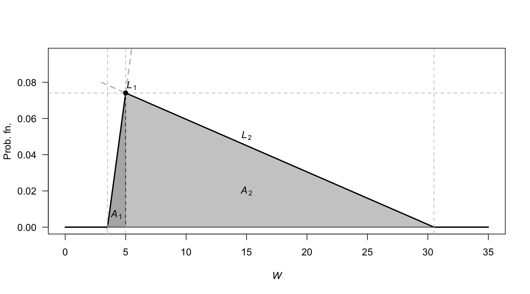
FIGURE F.30: Waiting times.

Answer for Exercise 5.23. Using the PMF from Exercise 4.28: \[ \operatorname{E}[X] = \left(0\times\frac{4}{10}\right) + \left(1\times\frac{3}{10}\right) + \left(2\times\frac{2}{10}\right) + \left(3\times\frac{1}{10}\right) = 1. \] In R:

set.seed(777023)

dist <- array(NA, dim = 1000)
for (i in (1:1000)){
  positions <- sample(1:5, size = 2, replace = FALSE)
  dist[i] = abs(diff(positions)) - 1
}
mean(dist)
#> [1] 0.926

Exercise 5.24.

Show by substituting.
Proceed: \[ \varphi(t) = \operatorname{E}[\exp(itX)] = \int_{\mathbb{R}} \exp(itx) f(x)\, dx. \] Differentiating wrt $t$: \[ \varphi(t)' = \int_{\mathbb{R}} ix \exp(itx) f(x)\, dx. \] Setting $t = 0$: \[ \varphi(0)' = \int_{\mathbb{R}} xi f(x)\, dx, \] and so $-i\varphi(0) = \operatorname{E}[X]$ as to be shown.

Exercise 5.25.

$(1 - a)^{-1} = 1 + a + a^2 + a^3 + \dots = \sum_{n=0}^\infty a^n$ for $|a| < 1$.
$(1 - tX)^{-1} = 1 + tX + t^2X^2 + t^3X^3 + \dots = \sum_{n=0}^\infty t^n X^n$ for $|tX| < 1$. Thus: \[\begin{align*} \operatorname{E}\left[ (1 - tX)^{-1}\right] &= \operatorname{E}[1] + \operatorname{E}[tX] + \operatorname{E}[t^2X^2] + \operatorname{E}[t^3X^3] + \dots\\ &= \sum_{n=0}^\infty \operatorname{E}\left[ t^n X^n\right] \quad \text{for $|tX| < 1$}. \end{align*}\]
Using the definition of an expected value: \[ R_Y(t) = \operatorname{E}\left[ (1 - tY)^{-1} \right] = \int_0^1 \frac{1}{1 - ty}\, dy = -\frac{\log(1 - t)}{t}. \]
Using the series expansion of $\log(1 - t)$: \[ \log(1 - t) = -t - \frac{t^2}{2} - \frac{t^3}{3} + \dots \] and so \[ -\frac{\log(1 - t)}{t} = 1 + \frac{t}{2} + \frac{t^2}{3} + \dots. \]
Equating this expression with that found in Part 2: \[\begin{align*} 1 + \frac{t}{2} + \frac{t^2}{3} + \dots. &= 1 + \operatorname{E}[tY] + \operatorname{E}[t^2 Y^2] + \operatorname{E}[t^3 Y^3] + \dots\\ &= 1 + t \operatorname{E}[Y] + t^2\operatorname{E}[Y^2] + t^3\operatorname{E}[Y^3] + \dots \end{align*}\] and so \[\begin{align*} t \operatorname{E}[Y] &= t/2 \Rightarrow \operatorname{E}[Y] = 1/2;\\ t^2 \operatorname{E}[Y^2] &= t^2/3 \Rightarrow \operatorname{E}[Y^2] = 1/3;\\ t^n \operatorname{E}[Y^n] &= t^n/(n + 1) \Rightarrow \operatorname{E}[Y^n] = 1/(n + 1).\\ \end{align*}\]

Exercise 5.26. First see that the area under the curve must be one, so \[ 1 = \int_{-c}^c k(3x^2 + 4)\, dx = k(2c^3 + 8c). \] Then, note that $\operatorname{E}[W] = 0$ (as the PDF is symmetric about 0), so that $\operatorname{var}[X] = \operatorname{E}[X^2]$, and: \[ \operatorname{E}[X^2] = \int_{-c}^c k x^2 (3x^2 + 4)\, dx = k c^3\frac{18c^2 + 40}{15} = \frac{28}{15}, \] and hence, equating the top lines of both fractions: \[ k c^3(9c^2 + 20) = 14. \] So we have two equations in two unknowns. Equating we obtain, after some algebra, \[ 9 c^4 - 8c^2 - 112 = 0. \] This is just a quadratic equation in $c^2$; so write \[ 9 X^2 - 8X - 112 = (9X + 28)(X - 4) = 0 \] with the two solutions $X = c^2 = -28/9$ (which has no real solutions for $c$), and $X = c^2 = 4$, so that $c = 2$ (as the PDF must be positive), giving $k = 1/32$.

Exercise 5.27. 1. $c = 1 - 3k/2$ and $c > 0$ and $k > 0$. 2. $c = k = 2/5$. 3. Not possible.

Exercise 5.28. $k = \infty$.

Exercise 5.29. $r = 5$.

Exercise 5.30. $\operatorname{E}[D] = \sum_{d=1}^9 \log_{10}\left(\frac{d + 1}{d}\right) \times d$. By expanding, and collecting like terms, and simplifying (e.g., $\log_{10} 1 = 0$ and $\log_{10}10 = 1$), find \[ \operatorname{E}[D] = -\log_{10}2 - \log_{10}3 - \cdots - \log_{10}8 - \log_{10}9 + 9 \approx 3.440. \]

Exercise 5.31.

TBA.
TBA.

FIGURE F.31: von Mises distribution.

Exercise 5.32.

TBA.

FIGURE F.32: inverse Gaussian distributions.

Exercise 5.33.

$\int_c^\infty c/w^3\, dy = 1/(2c)$ and so $c = 1/2$.
$\operatorname{E}[W] = \int_{1/2}^\infty w/(2w^3) \, dy = 1$.
$\operatorname{E}[W^2] = \int_{1/2}^\infty w^2/w^3\, dy$ which does not converge; the variance is undefined.

Exercise 5.34.

$k > 0$
Differentiating: $f_X(x) = \alpha k^\alpha x^{-\alpha - 1}$.
$\operatorname{E}[X] = \alpha k/(\alpha - 1)$. Also, $\operatorname{E}[X^2] = \alpha k^2/(\alpha - 2)$, and so $\operatorname{var}[X] = \alpha k^2/[(\alpha - 2)(\alpha - 1)^2]$.
No answer (yet).
See below.
$\Pr(X > 4 \cap X < 5) = \Pr(4 < X < 5) = F(5) - F(4) = (3/4)^3 - (3/5)^3 = 0.205875$. Also, $\Pr(X < 5) = 1 - (3/5)^3 = 0.784$. So the prob. is $0.205875/0.784 = 0.2625957$.
No answer (yet).

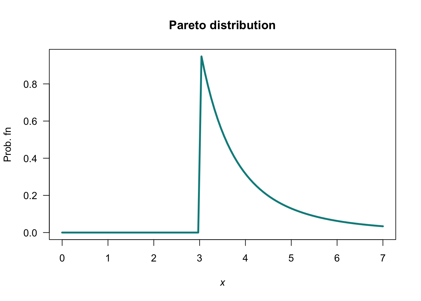
FIGURE F.33: A Pareto distribution

Exercise 5.36.

$\operatorname{E}[X] = \sum_{x = 1}^K x. p_X(x) = (1/6) + \sum_{x = 2}^K 1(x - 1)$. $\operatorname{E}[X^2] = \frac{1}{K} + \sum_{x=2}^K \frac{x}{x - 1}$ with no closed form, so the variance is a PITA. No closed form!
See Fig. F.34.
Applying the definition: \[ M_X(t) = \operatorname{E}[\exp(tX)] = \frac{1}{K} + \left( \frac{\exp(2t)}{2\times 1} + \frac{\exp(3t)}{3\times 2} + \frac{\exp(4t)}{4\times 3} + \dots + \frac{\exp(Kt)}{K\times (K - 1)}\right). \]

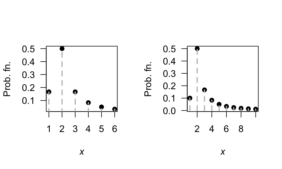
FIGURE F.34: The Soliton distribution.

Exercise 5.40.

Since $M_X(t) = \lambda/(\lambda - t)$, then $M_X(it) = \lambda/(\lambda - it)$. Then \[\begin{align*} f_X(x) &= \int_{-\infty}^{\infty} M_X(it) ] \exp(-itx)\, dt \\ &= \int_{-\infty}^{\infty} \frac{\lambda}{\lambda - it} (\cos(-tx) + \sin(-tx))\, dt\\ &= \int_{-\infty}^{\infty} \frac{\lambda(\lambda + it)}{\lambda^2 + t^2} (\cos(tx) - \sin(tx))\, dt \\ &= \int_{-\infty}^\lambda \frac{\lambda}{\lambda^2 + t^2} (\lambda\cos(tx) + t\sin(tx))\, dt. \end{align*}\]

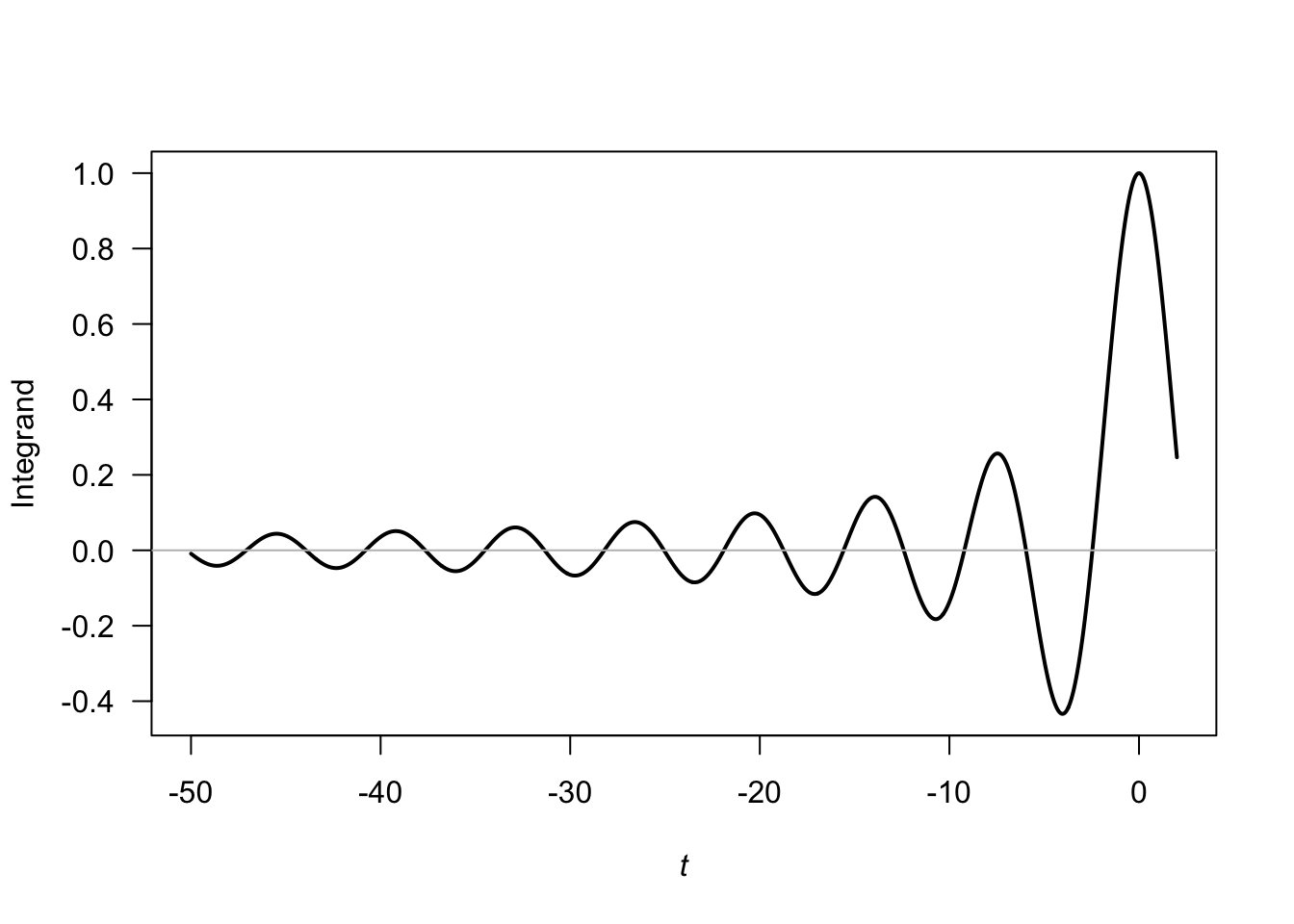
FIGURE F.35: The integrand.

Exercise 5.44.

$\operatorname{E}[X] = (n + 1) - n (1 - p)^n$.
$\operatorname{E}[X^2] = (n + 1)^2 n(n + 2)(1 - p)^n$, so $\operatorname{var}[X] = n^2(1 - p)^n[ 1 - (1 - p)^n]$.
As $p \to 0$ (i.e., no-one has the disease), the expected number of tests is one (with no variation). As $p \to 1$ (i.e., everyone has the disease), the expected number of tests is five (with no variation).
Using $\operatorname{E}[X] > n$, solve to find $p > 1 - (1/n)^{1/n}$.
Tests without pooling is $n$; expected number with pooling: $(n + 1) - n (1 - p)^n$. So the expected number of saved tests is See Fig. F.36.
With $n = 4$, the expected number of tests saved is $4 - (5 - 4(1-p)^4) \approx 1.6244$. So doing this $50$ times (i.e., $50 \times 4 = 200$) would save $50\times 1.6244 \times 15 = 1218.3$; about 1220 in cost savings.
$\Pr(\text{Need individual tests})$ ${}={}$ $\Pr(\text{Pooled test is positive})$ ${}={}$ $1 - \Pr(\text{Pooled test is negative})$ ${}={}$ $1 - \Pr(\text{All individuals are negative})$ ${}={}$ $1 -(0.9)^ 4 = 0.3439$. So the PMF of $N$, the number of tests needed, is \[ p_N(n) = \begin{cases} 0.6561 & \text{for $n = 1$ (i.e., pooled test only)};\\ 0.3439 & \text{for $n = 5$ (i.e., one pooled test, olus four individual tests)} \end{cases} \] Then $\operatorname{E}[X] = (0.6561 \times 1) + (0.3439 \times 5) = 2.3756$ and $\operatorname{E}[X^2] = (0.6561 \times 1^2) + (0.3439 \times 5^2) = 9.2536$ so that $\operatorname{var}[X] = 3.610125$. So for a pool of four people, rather than four tests we would expected to have to conduct $2.3756$ tests, a saving of $4 - 2.3756 = 1.6244$ tests.

If $200$ people in total, testing each individual would cost $200\times 15 = \$3000$. With $n = 4$, a total of $50$ pools are created, and each pool saves $1.6244$ tests, so the total number of tests expected to be saved in $50 \times 1.6244 = 81.22$; at $15 each, the saving is $\$1218.30$.

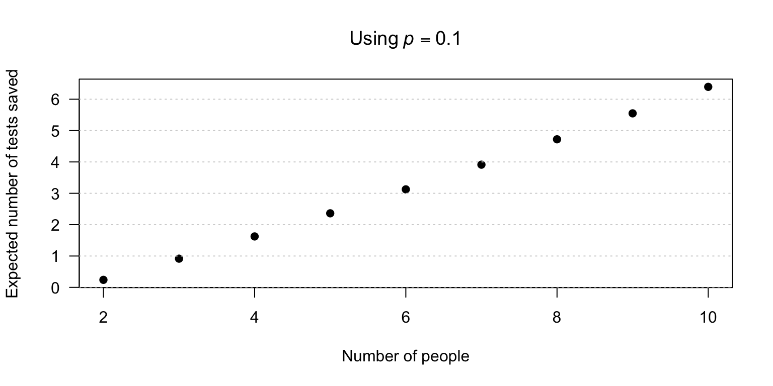
FIGURE F.36: The expected number of tests saved by pooling.

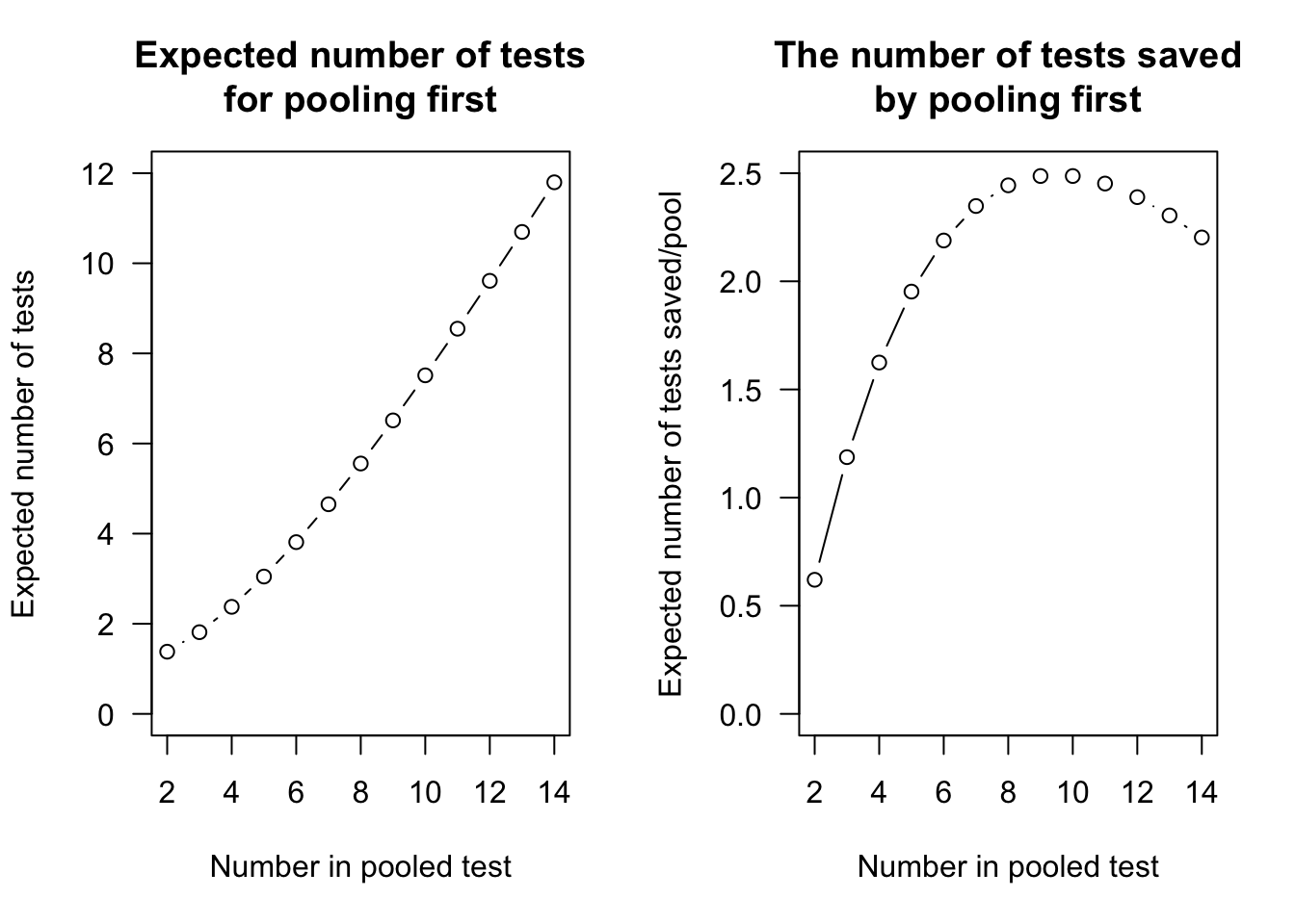
FIGURE F.37: The advantage of initial pooled testing.

Exercise 5.46.

$\operatorname{E}[X] = 7/2$.
$\operatorname{MAD}[X] = 1.5$.

Exercise 5.49.

Plot not shown, but a quadratic symmetric about $x = 0$.
All odd moments are zero since distribution symmetric: $\operatorname{E}[X] = 0$. $\operatorname{var}[X] = \operatorname{E}[X^2] = 3/5$.
Odd moment, and distribution obviously symmetric; skewness is zero.
$\operatorname{E}[X^4] = 3/7$, so kurtosis is $\mu_4/\mu^2_2 = (3/7)/(3/5)^2 = 25/21$. Hence, the excess kurtosis is $25/21 - 3 = -38/21$.
No values in the extreme values like a normal; all values are contained within $-1 < x < 1$.

Exercise 5.50.

Plot not shown, but straight line from $(0, 0)$ to $(2, 1)$.
$\operatorname{E}[X^r] = 2^{r + 1}/(r + 2)$.
$\operatorname{E}[X] = 4/3$; $\operatorname{var}[X] = 2 - (4/3)^2 = 14/9$.
$\operatorname{E}[ (X - \mu)^3] = -8/135$, so skewness is $\mu_3 / \mu_2^{3/2} = (-8/135)/(14/9)^{3/2} = -2\sqrt{14}/245$. Negative value: left skewed; bulk of probability to the right side.
$\operatorname{E}[(X - \mu)^4] = 16/135$, so kurtosis is $\mu_4/\mu^2_2 = (16/135)/(14/9)^2 = 12/245$. Hence, the excess kurtosis is $12/245 - 3 = -723/245$ No values in the extreme values like a normal; all values are contained within $0 < x < 2$.

Exercise 5.51. $\varphi_X(t) = \exp(-|t|)$.

Exercise 5.52. TBA.

Exercise 5.53. TBA.

Exercise 5.54. TBA.

Exercise 5.55. Let $D = 1$ if defective (prob $0.1$), $D = 0$ otherwise.

$\operatorname{E}[C] = \operatorname{E}[C\mid D=1]\cdot 0.1 + 0 = 100 \times 0.1 = 10$.
$\operatorname{E}[\operatorname{var}[C\mid D]] = 0.1 \times \operatorname{var}[\text{Gamma}(2,50)] + 0.9\times 0 = 0.1\times 5000 = 500$; $\operatorname{var}[\operatorname{E}[C\mid D]] = 0.1\times(100-10)^2 + 0.9\times(0-10)^2 = 810 + 90 = 900$. So $\operatorname{var}[C] = 1400$.

Exercise 5.56.

$\operatorname{E}[F] = (0.15\times 8) + (0.85\times 0) = 1.2$.
$\operatorname{E}[\operatorname{var}[F\mid D]] = 0.15\times 25 = 3.75$. $\operatorname{var}[\operatorname{E}[F\mid D]] = 0.15\times(8 - 1.2)^2 + 0.85\times(0 - 1.2)^2 = 6.936 + 1.224 = 8.16$. $\operatorname{var}[F] = 11.91$.

Exercise 10.20.

$\operatorname{E}[U] = 4 3 = 1$; $\operatorname{E}[V] = 2 + 6 = 8$.
$\operatorname{var}[U] = 4\times4 + 9 - 2\times2\times3 = 16 + 9 - 12 = 13$; $\operatorname{var}[V] = 4 + 4\times9 + 2\times2\times3 = 4 + 36 + 12 = 52$.
$\operatorname{Cov}(U,V) = \operatorname{Cov}(2X-Y, X+2Y) = 2\operatorname{var}[X] + 4\operatorname{Cov}(X,Y) - \operatorname{Cov}(Y,X) - 2\operatorname{var}[Y] = 8+12-3-18 = -1$.
$\operatorname{Corr}(U,V) = -1/\sqrt{13\times52} = -1/26$.

Exercise 10.21.

$\operatorname{E}[S] = -1 + 12 = 11$; $\operatorname{E}[T] = -2 - 4 = -6$.
$\operatorname{var}[S] = 9 + ( + 2\times 3 \times (-2) = 6 = 6$; $\operatorname{var}[T] = 36 + 1 - 2\times 2\times (-2) = 45$.
$\operatorname{Cov}(S, T) = \operatorname{Cov}(X + 3Y, 2X - Y) = 2\times9 - 9 + 6\times(-2) - 3\times(-2)\times(-1)...$; working through: $= 2\operatorname{var}[X] - \operatorname{Cov}(X,Y) + 6\operatorname{Cov}(X,Y) - 3\operatorname{var}[Y] = 18+5\times(-2)-3 = 18-10-3=5$.
$\operatorname{Corr}(S, T) = 5/\sqrt{6\times45} = 5/\sqrt{270}\approx 0.304$.

Exercise 5.59.

$970 < X < 1030$ means $|X - 1000| < 30 = 3\sigma$, so $k=3$ and $\Pr(|X - \mu|<3\sigma)\geq 1 - 1/9 = 8/9 \approx 0.889$.
$|X - 1000| > 25 = 2.5\sigma$, so $\Pr(\text{rejected}) \leq 1/2.5^2 = 0.16$.

Exercise 5.60.

$k = 8/\sigma = 8/4 = 2$, so $\Pr(|X - 20|\ge 8) \le 1/4 = 0.25$. 1, $1/k^2 \le 0.04$ gives $k\ge 5$, so $k\sigma = 5\times 4= 20$: $\Pr(|X - 20| \ge 20) \le 0.04$.

Exercise 5.61.

Differentiating: $\kappa_1 = \mu$, $\kappa_2 = \sigma^2$, $\kappa_3 = 0$ and $\kappa_4 = 0$.
$\gamma_1 = \kappa_3/\kappa_2^{3/2} = 0$; $\gamma_2 = \kappa_4/\kappa_2^2 = 0$.

Exercise 5.62.

$K'_X(t) = \lambda \exp(t)$, so $\kappa_r = \lambda$ for all $r \ge 1$.
$\gamma_1 = \lambda/\lambda^{3/2} = 1/\sqrt{\lambda}$; $\gamma_2 = \lambda/\lambda^2 = 1/\lambda$.

Exercise 5.63.

Differentiating twice, $g'(x) = 1/x$ and $g''(x) = -1/x^2 < 0$ for all $x > 0$. Since the second derivative is everywhere negative, $g$ is strictly concave.
Since $g(x) = \log x$ is strictly concave, Jensen’s inequality reverses: \[ \operatorname{E}[g(X)] \leq g(\operatorname{E}[X]), \] that is, \[ \operatorname{E}[\log X] \leq \log \operatorname{E}[X] = \log \mu, \] with equality if and only if $X$ is degenerate.
For $X \sim \operatorname{Exponential}(\lambda)$, we have $\operatorname{E}[X] = 1/\lambda$, so \[ \log(\operatorname{E}[X]) = \log\frac{1}{\lambda} = -\log\lambda. \] To compute $\operatorname{E}[\log X]$, we use the PDF $f(x) = \lambda e^{-\lambda x}$ for $x > 0$: \[ \operatorname{E}[\log X] = \int_0^\infty (\log x)\,\lambda e^{-\lambda x}\,\mathrm{d}x. \] Using the substitution $u = \lambda x$ and the known result $\int_0^\infty (\log u)\, e^{-u}\,du = -\gamma$, where $\gamma \approx 0.5772$ is the Euler–Mascheroni constant, \[ \operatorname{E}[\log X] = \int_0^\infty \log\!\left(\frac{u}{\lambda}\right) e^{-u}\,du = \int_0^\infty (\log u)\,e^{-u}\,du - \log\lambda = -\gamma - \log\lambda. \] Since $\gamma > 0$, we have $\operatorname{E}[\log X] = -\gamma - \log\lambda < -\log\lambda = \log(\operatorname{E}[X])$, confirming the strict inequality from part (b).

Exercise 5.64.

For fixed $t$, let $g(x) = e^{tx}$. Then $g''(x) = t^2 e^{tx} > 0$ for all $x$ and all $t \neq 0$, so $g$ is strictly convex. By Jensen’s inequality, \[ \operatorname{E}[e^{tX}] \geq e^{t\operatorname{E}[X]} = e^{t\mu}, \] with equality if and only if $X$ is degenerate. For $t = 0$ both sides equal $1$ trivially.
Since $\log$ is a strictly increasing function and $M_X(t) \geq e^{t\mu}$ from part 1., \[ \log M_X(t) \geq \log e^{t\mu} = t\mu. \]
Differentiating $K_X(t) = \log M_X(t)$, \[ K_X'(t) = \frac{M_X'(t)}{M_X(t)}. \] At $t = 0$, $M_X(0) = 1$ and $M_X'(0) = \operatorname{E}[X] = \mu$, so \[ K_X'(0) = \frac{\mu}{1} = \mu. \] The result of part 2. says $K_X(t) \geq t\mu = tK_X'(0)$, which states that the cumulant generating function lies above its tangent line at $t = 0$. This is precisely the condition that $K_X$ is convex at the origin, consistent with the general result that cumulant generating functions are convex wherever they exist.

Exercise 5.7.

$\operatorname{E}[X] = 0.4$.
$\operatorname{E}[X^2] = 0.8$ so $\operatorname{var}[X] = 0.64$.
$M_X(t) = 0.6 + \frac{0.4}{1 - t}$ if $t < 1$.
$M'_X(t) = \frac{0.4}{(1 - t)^2}$ so $M_X'(0) = 0.4$. $M''_X(t) = \frac{0.8}{(1 - t)^3}$ so $M_X''(0) = 0.8$ as above.

Exercise 5.8.

$\operatorname{E}[R] = 0\times \Pr(R = 0) + \int_{0.1}^{70} r\, f_X(r)\, dr + 70\times \Pr(R \ge 70) \approx 19.396$.
$\operatorname{E}[R^2] \approx 691.298$ so $\operatorname{var}[R] \approx 315.092$.
$M_X(t) = \frac{1}{1 - 20t}$ if $t < 1/20$. $M_R(t) = 1 - \exp(-0.005) + \int_{0.1}^{70} \exp(tx) \frac{\exp(-x/20)}{20}\,dx + \exp(70t) \exp(-3.5)$. (This becomes $1 - \exp(-0.005) + \frac{\exp(70(t - 1/20)) - \exp(0.1(t - 1/20))}{20(t - 1/20)} + \exp(70t - 3.5)$.)

F.5 Answers for Chap. 6

Exercise 6.1.

Discrete Uniform: all outcomes from $1$ to $6$ are equally likely.
Bernoulli: single trial with two outcomes (success; failure).
Poisson: counts events in a fixed time interval with random arrivals.

Exercise 6.2.

Binomial: fixed number of independent trials, counting successes.
Geometric: number of trials until first success.
Hypergeometric: sampling without replacement from a finite population.

Exercise 6.3.

Poisson: counts events occurring randomly in a fixed time interval.
Hypergeometric: sampling without replacement from a finite population.
Negative binomial: number of trials needed to achieve a fixed number (4) of failures (or successes), with independent repeated trials.

Exercise 6.4.

Poisson: counts arrivals over time with a constant rate.
Geometric: trials until the first success.
Binomial: sampling with replacement gives independent trials with fixed probability of defect.

Exercise 6.13. From what is given: $p_X(x; n, 1 - p) = \binom{n}{x} (1 - p)^x p^{n - x}$. Then, define $Y = n - X$ and hence $f_Y(y) = \binom{n}{y} p^y (1 - p)^{n - y}$, which is $f_Y(y) = \binom{n}{n - x} p^{n - x} (1 - p)^{n}$. It is easy to show $\binom{n}{x} = \binom{n}{n - x}$ and hence $f_X(x)$ and $f_Y(y)$ are equivalent.

Exercise 6.5. Care: The geometric is parameterised so that $x$ is the number of failures before a success (not the number of trails). Similarly for the negative binomial.

sum( dbinom(10:25, # Part 1
            size = 25, prob = 0.30) )
#> [1] 0.189436
sum( dbinom(0:9,  # Part 2
            size = 25, prob = 0.30) )
#> [1] 0.810564
sum( dbinom(5:10,  # Part 3
            size = 25, prob = 0.30) )
#> [1] 0.8117281
dgeom(x  = 5,  # Part 4: 5 fails before 1st success
      prob = 0.30)
#> [1] 0.050421

sum( dgeom(x  = 7:50,  # Part 5: Num. fails! 
           prob = 0.30) )
#> [1] 0.08235429

# Part 6; This means 5 fails, before 3rd success
dnbinom(x = 5, prob = 0.30, size = 3)
#> [1] 0.09529569

Assumes independence of people, and a constant probability.

Exercise 6.7. Take care: The geometric and negative binomials are parameterised so that $x$ is the number of failures before a success (not the number of trails).

sum( dbinom( 16:81,  # Part 1
             size = 81, prob = 0.20) ) 
#> [1] 0.5663638
sum( dbinom( 12:81,  # Part 2
             size = 81, prob = 0.20) ) 
#> [1] 0.9082294
  # Part 3
dgeom(x = 2, #i.e., two failures before first success
      prob = 0.20)
#> [1] 0.128

  # Part 4
dnbinom(x = 5, # is 5 fails before 5th success
        prob = 0.20, size = 5) 
#> [1] 0.01321206
sum( dbinom(50:81, size = 81, prob = 0.2) )
#> [1] 3.042983e-16

Exercise 6.8. TBA.

Exercise 6.9.

dpois( 0, lambda = 3)
#> [1] 0.04978707
sum( dpois( 6:50, lambda = 3) )
#> [1] 0.08391794
dpois( 2, lambda = 6)
#> [1] 0.04461754

Exercise 6.11.

See Fig. F.38.

#> [1] 0.1252978
#> [1] 0.2424239
#> [1] 0.3401473
#> [1] 0.5232259

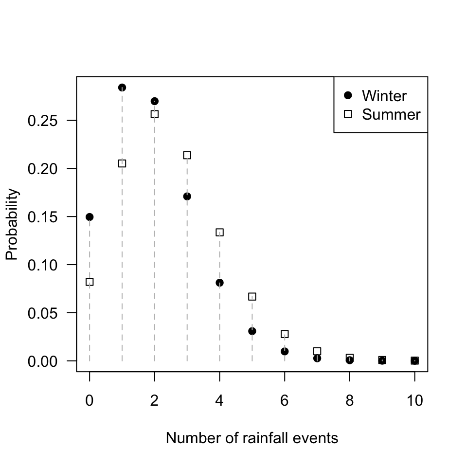
FIGURE F.38: The number of rainfall events in summer and winter.

Exercise 6.12.

Yep.
$\log n_x = \log N + \log p + x\log (1 - p)$, which is a linear regression model of $\log n_x$ regressed on $x$, with intercept $\beta_0 = \log N + \log p$ and slope $\beta_1 = \log (1 - p)$.
So from the fitted slope, we can estimate $p$; then, using the estimated intercept, we can estimate $N$. More specifically, the estimate of $p$ is $1 - \exp( \hat{\beta}_1)$, and the estimate of $N$ is then $\exp(\beta_0 - \log p)$. We find $\hat{y} = 6.40525 - 1.128753x$. Then, the population size is estimate as about $894$: $p = 0.6765636$. $N = 894.2445$.

x <- 1:6
nx <- c(247, 63, 20, 4, 2, 1)

m1 <- lm( log(nx) ~ x); coef(m1)
#> (Intercept)           x 
#>    6.405250   -1.128753
beta0 <- coef(m1)[1]
beta1 <- coef(m1)[2]

p <- 1 - exp(beta1); p
#>         x 
#> 0.6765636
N <- exp(beta0 - log(p) ); N
#> (Intercept) 
#>    894.2445

Exercise 6.14 Defining $X$ as the ‘number of failures until $4$kWh/m² was observed’, since the parameterisation used in the textbook is for the number of failures until the first success. Then, $X\sim \text{Geom}(p)$.

$\operatorname{E}[X] = (1 - p)/p = 1$ failures till first success, followed by the day of success: so $2$.
$\operatorname{E}[X] = (1 - p)/p = 3$ failures, so $3 + 1 = 4$.
$\operatorname{var}[X] = (1 - p)/p^2 = 12$.

# Part 4
sum( dgeom(0:2,  # 0 to 2 failures before the success
           prob = 0.25))
#> [1] 0.578125

Exercise 6.20.

See Fig. F.39; not hugely different.
Similar probabilities: $0.85$ (in 1999) and $0.91$ (in 2000).
Similar: $16$ days (in 1999) and $12$ (in 2000).
Writing $X$ for the clutch size (where $n = 237$):
- $\operatorname{E}[X] = (1\times \frac{9}{237}) + (2\times \frac{29}{237}) + (3\times \frac{199}{237}) = 2.801688$, or about 2.8.
- $\operatorname{E}[X^2] = (1^2\times \frac{9}{237}) + (2^2\times \frac{29}{237}) + (3^2\times \frac{199}{237}) = 8.084388$.
- So, $\operatorname{var}[X] = 8.084388 - (2.801688)^2 = 0.2349324$, so the standard deviation is 0.4846982, or about 0.485.

  ## Part 2
1 -  pnbinom(30, mu = 23.0, size = 20.6) # 0.1416996
#> [1] 0.1416996
1 - pnbinom(30, mu = 19.5, size = 8.9) # 0.09175251
#> [1] 0.09175251
  ## Part 3
qnbinom(0.15, mu = 23.0, size = 20.6) # 16
#> [1] 16
qnbinom(0.15, mu = 19.5, size = 8.9)  # 12
#> [1] 12

x <- 0:50
y1999 <- dnbinom(x, mu = 23.0, size = 20.6)
y2000 <- dnbinom(x, mu = 19.5, size = 8.9)

plot( y1999 ~ x,
      pch = 19, las = 1,
      main = "Lay date for glaucous-winged gulls",
      xlab = "Lay date",
      ylab = "Prob. function")
points( y2000 ~ x, pch = 1)
legend("topleft", pch = c(19, 1),
       legend = c("1999", "2000"))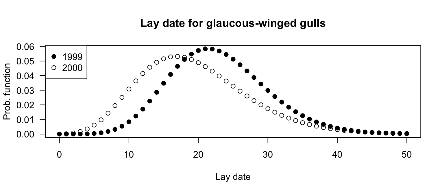

FIGURE F.39: The lay-date model for glaucous-winged gulls, in 1999 and 2000

Exercise 6.21. In Eq. (6.7), the rv $X$ refers to the number of failures before the $r$th success is observed, so that $X = 0, 1, 2, \dots$. So define $Y$ as the number of trials till the $r$th success, and hence $Y = X + r$.

The range is $Y\in\{r, r + 1, r + 2, \dots\}$
$p_Y(y; p, r) = \binom{y - 1}{r - 1}(1 - p)^{y - r} p^{r - 1}$, for $y = r, r + 1, r + 2, \dots$.
$\operatorname{E}[Y] = \operatorname{E}[X + r] = \operatorname{E}[X] + r = r/p$.
$\operatorname{var}[Y] = \operatorname{var}[X + r] = \operatorname{var}[X] = r(1 - p)/p^2$.

Exercise 6.22. Let $X$ be the number of typos per minute; then $X\sim\text{Poisson}(\lambda = 2.5\times 5 = 12.5)$ for a five-minute test.

dpois(10, lambda = 12.5) # 0.09564364
#> [1] 0.09564364
dpois(6, lambda = 2.5 * 3) * dpois(4, lambda = 2.5 * 2) #  0.02398959
#> [1] 0.02398959

For Part 3: The number of errors occurring in the ‘overlap minute’ could be $0, 1, 2, \dots 6$. So proceed:

$6$ errors in overlap minute: $\Pr(\text{0 errors first 2 mins})\times{}$ $\Pr(\text{6 errors overlap min})\times{}$ $\Pr(\text{0 errors final 2 mins})$
$5$ errors in overlap minute: $\Pr(\text{1 error first 2 mins})\times{}$ $\Pr(\text{5 errors overlap min})\times{}$ $\Pr(\text{1 error final 2 mins})$

And so on.

prob <- function(ErrorsInOverlap){
  dpois( (6 - ErrorsInOverlap), lambda = 2 * 2.5) *
  dpois(ErrorsInOverlap, lambda = 1 * 2.5) *
  dpois((6 - ErrorsInOverlap), lambda = 2 * 2.5)
}
sum( prob( 0:6 ) ) # 0.02120811
#> [1] 0.02120811

Exercise 6.23.

$0.25$.
dbinom(x = 2, size = 4, prob = 0.25) ${}= 0.2109375$.

Exercise 6.24. The code below is for one simulation for each part only.

### Part 1
set.seed(2268) # For reproducibility

queueLength <- array(dim = 60)
queueLength[1] <- rpois(1, lambda = 0.5)

for (i in 2:60){
   queueLength[i] <- queueLength[i - 1] + rpois(1, lambda = 0.5)
   # Print every 10 minutes
   if ( floor(i/10) == i/10 ) {
     cat("After ", i, " minutes past 8AM, queue length: ", queueLength[i], "\n")
   }
}
#> After  10  minutes past 8AM, queue length:  6 
#> After  20  minutes past 8AM, queue length:  14 
#> After  30  minutes past 8AM, queue length:  19 
#> After  40  minutes past 8AM, queue length:  24 
#> After  50  minutes past 8AM, queue length:  28 
#> After  60  minutes past 8AM, queue length:  34
plot( queueLength, type = "l", las = 1, lwd = 3)

FIGURE F.40: A simulation


### Part 2
queuelength <- array(dim = 60)
queueLength[1] <- rpois(1, lambda = 0.5)

for (i in 2:60){
   NumberIn <- rpois(1, lambda = 0.5)

   # Number being served
   if ( i < 30 ) {
     NumberServed <- 0
   } else {
     if (i >= 30) {
        lambda <- 0.75
     }
     NumberServed <- rpois(1, lambda = lambda)
     queueLength[i] <- queueLength[i - 1] + NumberIn - NumberServed
   }
   if ( queueLength[i] < 0 ) queueLength[i] <- 0
}

plot( queueLength, type = "l", las = 1)
abline(v = 30, lwd = 3)
text(30, 5, pos = 3, # To the right,
     labels = "Server starts")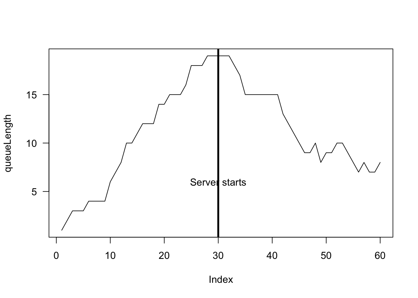

FIGURE F.41: A simulation


### Part 3.
queuelength <- array(dim = 60)
queueLength[1] <- rpois(1, lambda = 0.5)

for (i in 2:60){
   NumberIn <- rpois(1, lambda = 0.5)

   # Number being served
   if ( i < 30 ) {
     NumberServed <- 0
   } else {
     if ( (i > 30) & (i < 45) ) {
        lambda <- 0.7
     }
     if ( i > 45 ) {
        lambda <- 1.3
     }
     NumberServed <- rpois(1, lambda = lambda)
   }

   queueLength[i] <- queueLength[i - 1] + NumberIn - NumberServed
   if ( queueLength[i] < 0 ) queueLength[i] <- 0
}

plot( queueLength, type = "l", las = 1, lwd = 3)
abline(v = 30, lwd = 2, col = "grey")
text(30, 5,
     pos = 3, # To the right,
     labels = "Server 1 starts")
abline(v = 45, lwd = 2, col = "grey")
text(45, 5,
     pos = 3, # To the right,
     labels = "Server 2 starts")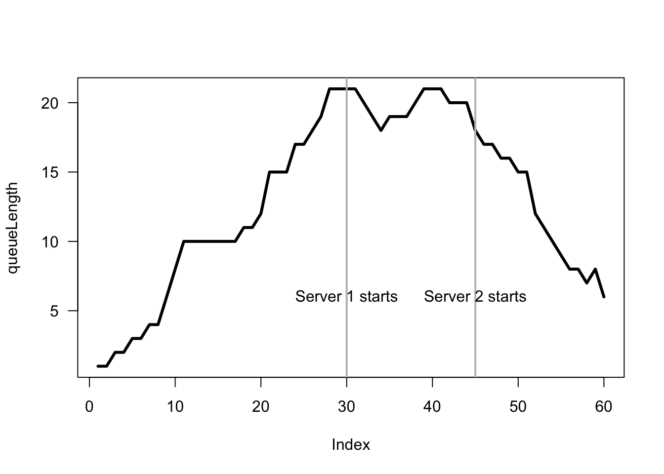

FIGURE F.42: A simulation

Exercise 6.25. Suppose $X\sim\text{Poisson}(\lambda)$; then $\Pr(X) = \Pr(X + 1)$ implies \[\begin{align*} \frac{\exp(-\lambda)\lambda^x}{x!} &= \frac{\exp(-\lambda)\lambda^{x + 1}}{(x + 1)!} \\ \frac{\lambda^x}{x!} &= \frac{\lambda^{x} \lambda}{(x + 1) \times x!} \end{align*}\] so that $\lambda = x + 1$ (i.e., $\lambda$ must be a whole number). For example, if $x = 4$ we would have $\lambda = 5$. And we can check:

dpois(x = 4,     lambda = 5)
#> [1] 0.1754674
dpois(x = 4 + 1, lambda = 5)
#> [1] 0.1754674

Exercise 6.26.

$\operatorname{E}[X] = kp$ which is the same as the binomial (here, $k$ is the sample size).
$\operatorname{var}[X] = k p (1 - p) \times \left(\frac{N - k}{N - 1}\right)$; the first bit is the variance for the binomial distribution (recall $k$$ is the sample size). The other term is $(N - k)/(N - 1)$, which is the FPC factor as defined.

Exercise 6.27. Since $\operatorname{var}[Y] = \operatorname{E}[Y^2] - \operatorname{E}[Y]^2$, find $\operatorname{E}[Y^2]$ using (B.2): \[\begin{align*} \operatorname{E}[Y^2] &= \sum_{i = 0}^{b - a} i^2\frac{1}{b - a + 1}\\ &= \frac{1}{b - a + 1}(0^2 + 1^2 + 2^2 + \dots +(b - a)^2)\\ &= \frac{1}{b - a + 1}\frac{(b - a)(b - a + 1)(2(b - a) + 1)}{6}\\ &= \frac{(b - a)(2(b - a) + 1)}{6}. \end{align*}\] Therefore \[ \operatorname{var}[X] = \operatorname{var}[Y] = \frac{(b - a)(2(b - a) + 1)}{6} - \left(\frac{b - a}2\right)^2 = \frac{(b - a)(b - a + 2)}{12}. \]

Exercise 6.31. Let $Y = N - X$ be the number of Type B arrivals. $Y$ depends on $N$, so we sum over all possible vaues of $n$ (note: for $Y = k$, $N > k$): \[ \Pr(Y = k) = \sum_{n = k}^{\infty} \Pr(Y = k\mid N = n)\cdot \Pr(N = n). \] Given $N = n$, the number of Type B arrivals has a binomial distribution $\text{Binomial}(n, 1 - p)$, and $N$ follows a Poisson distribution. Hence, on substituting, \[ \Pr(Y = k) = \frac{\exp(-\lambda) (\lambda(1-p))^k}{k!} \sum_{m=0}^\infty \frac{(\lambda p)^m }{m!}, \] and the summation is the Taylor series expansion for $\exp(\lambda p)$, so we obtain \[ \Pr(Y = k) = \frac{\exp(-\lambda) (\lambda (1-p))^k}{k!} \exp(\lambda p) = \frac{\exp(-\lambda)(1-p)) (\lambda(1 - p))^k}{k!}, \] which is the PMF of a Poisson distribution, with parameter $\lambda(1 - p)$.

Exercise 6.32.

$\Pr(G_A = 0\text{\ and\ }G_H = 0) = \Pr(G_A = 0) \cdots \Pr(G_H = 0)$ by independence:

lamH <- 1.5; lamA <- 1.0

# Part 1
dpois(0, lamH) * dpois(0, lamA)
#> [1] 0.082085

# Part 2
1 - ppois(1, lamH)
#> [1] 0.4421746

# Part 3
p_draw <- 0
for (i in 0:10){
  p_draw <- p_draw + dpois(i, lamA) * dpois(i, lamH)  
}
cat("The probability of a draw:", p_draw, "\n")
#> The probability of a draw: 0.2598474

# Part 4
p_five <- 0
for (i in 0:5){
  p_five <- p_five + dpois(i, lamA) * dpois(5 - i, lamH)  
}
cat("The probability of five match-goals:", p_five, "\n")
#> The probability of five match-goals: 0.06680094

# Part 5
p_home_win <- 0
for (i in 1:10){ # To win, a team need at least one goal.
  for (j in (0:i)){
    p_home_win <- p_home_win + dpois(i, lamA) * dpois(j, lamH)  
  }
}
cat("The probability of home-team win:", p_home_win, "\n")
#> The probability of home-team win: 0.4299693

# Part 6
num_sims <- 2000
home_goals <- rpois(num_sims, lamH)
away_goals <- rpois(num_sims, lamA)
hist(home_goals + away_goals, freq = FALSE,
     las = 1, xlab = "Total goals",
     main = "Total game goals")

Exercise 6.33.

CHECK!!!!

p_home <- 0.90; p_away <- 0.85

# Part 1
cat("Prob home team makes all 5 shots:", dbinom(5, size=5, prob=p_home), "\n")
#> Prob home team makes all 5 shots: 0.59049

# Part 2
cat("Prob away team makes more than 3 shots:", 1 - pbinom(4, size=5, prob=p_home), "\n")
#> Prob away team makes more than 3 shots: 0.59049

# Part 3
cat("Prob away team's first on 2nd shot:", dgeom(2, p_away), "\n")
#> Prob away team's first on 2nd shot: 0.019125

# Part 4
cat("Prob away team's third goal on 5th shot:", dnbinom(5, 5, p_away), "\n")
#> Prob away team's third goal on 5th shot: 0.004245428

# Part 5
cat("Prob both team's fouth goal on 5th shot:", 
    dnbinom(4, 5, p_away) * dnbinom(4, 5, p_home), "\n")
#> Prob both team's fouth goal on 5th shot: 6.499326e-05

# Part 6
p_same <- 0
for (g in (0:5)){
  p_same <- p_same + dbinom(g, 5, p_home) * dbinom(g, 5, p_away)
}
cat("Prob same number goals:", p_same, "\n")
#> Prob same number goals: 0.4007083

# Part 7
p_home_win <- 0
for (gh in (1:5)){ # To win, must score at least one goal
  for (ga in (0:(gh-1))){ # To win, must score at least one goal
    p_home_win <- p_home_win + dbinom(gh, 5, p_home) * dbinom(ga, 5, p_away)
  }
}
cat("Prob home team wins shoot-out:", p_home_win, "\n")
#> Prob home team wins shoot-out: 0.3845039

Exercise ??.

The sudden-death shoot-out produces a winner if one teams scores a pgoal, and the other does not. So, the probability that any single round produces a winner is \[ q = p_H(1 - p_A) + (1 - p_H) p_A = (0.80\times 0.25) + (0.20\times 0.75) = 0.35. \] So each round of sudden-death could end the shoot-out, with probability $q = 0.35$.

Let $X$ denote the number of additional sudden-death rounds before the shoot-out ends, where $X = 1, 2, \dots$. This is the alternative parameterisation of the geometric distribution (Sect. 6.5.3). To use the parameterisation used in R, define $Y = X - 1$ so that $Y = 0, 1, 2, \dots$. Then, \[ Y\sim\text{Geometric}(p), \]

where $p = 0.35$.

The prob the shoot-out end in the first round is just $0.35$.
dgeom(2, prob = 0.35) or about $0.1479$.
pgeom(3, prob = 0.35, lower.tail = FALSE) or about $0.1785$.
For a geometric distribution, $\operatorname{E}[Y] = 1/p = 1/0.35 \approx 2.857$.
0.80*(1-0.75)/0.35, or approx. $0.5714$.

num_sims <- 10000
pA <- 0.80; pB <- 0.75

rounds <- numeric(num_sims)
A_wins <- logical(num_sims)

for (i in 1:num_sims) {
  r <- 0
  finished <- FALSE
  while (!finished) {
    r <- r + 1
    A <- rbinom(1, 1, pA)
    B <- rbinom(1, 1, pB)

    if (A != B) {
      rounds[i] <- r
      A_wins[i] <- (A == 1)
      finished <- TRUE
    }
  }
}

cat("Mean number of rounds:", mean(rounds), "\n")
#> Mean number of rounds: 2.8084
cat("P(Team A wins):", mean(A_wins), "\n")
#> P(Team A wins): 0.5698

F.6 Answers for Chap. 7

Exercise 7.1.

Beta: bounded between $0$ and $1$, modelling proportions.
Exponential: memoryless waiting time with constant hazard rate.
Gamma: sum of multiple service/waiting stages, giving total waiting time.

Exercise 7.2.

Normal: symmetric variation around a mean from many small additive effects.
Gamma: waiting time until multiple Poisson events occur (accumulated waiting time).
Log-normal: positive, right-skewed quantities formed by multiplicative effects.

Exercise 7.3.

Beta: models a random proportion bounded in $[0, 1]$.
Gamma: sum of multiple exponential waiting times (waiting for multiple events).
Normal: symmetric fluctuations around a mean, appropriate for small additive changes.

Exercise 7.4.

Exponential: waiting time between Poisson events with constant rate.
Log-normal: positive, right-skewed data from multiplicative processes.
Log-normal: environmental concentrations typically arise from multiplicative variation and are strongly right-skewed.

Exercise 7.19.

For example: From $\mu = m/(m + n)$, we get $n = m(1 - \mu)/\mu$ and $m + n = m/\mu$. Also, from the expression for the variance, substitute $m + n = m/\mu$ and simplify to get \[ n = \frac{\sigma^2 m (m + \mu)}{\mu^3} \] Equate this expression for $n$ with $n = m(1 - \mu)/\mu$ from earlier, and solve for $m$. We get that $m = \frac{\mu}{\sigma^2}\left( \mu(1 - \mu) - \sigma^2\right)$; $n = \frac{1 - \mu}{\sigma^2}\left( \mu(1 - \mu) - \sigma^2\right)$.

Exercise 7.20.

$\operatorname{E}[X] = (72 + 30)/2 = 51$km.h^$-1$. $\operatorname{var}[X] = (72 - 30)^2 / 12 = 147$(km.h^$-1$)^$2$ (more easily understood, as $\sqrt{\operatorname{var}[X]} = 12.12$km.h^$-1$).
See Fig. F.43.
See below; $2/7 \approx 0.2857$.
See below; $7/12 \approx 0.5833$.

1 - punif(60, 30, 72)
#> [1] 0.2857143
(1 - punif(65, 30, 72) ) /
  (1 - punif(60, 30, 72) )
#> [1] 0.5833333

par(mfrow = c(1, 2))

x <- seq(10, 100, length = 1000)
plot( x = x,
      y = dunif(x, min = 30, max = 72),
      type = "l", las = 1, lwd = 3,
      xlab = "Vehicle speeds (in km/h)",
      ylab = "Probability density",
      main = "PDF for vehicle speeds")

x <- seq(10, 100, length = 1000)
plot( x = x,
      y = punif(x, min = 30, max = 72),
      type = "l", lwd = 3, las = 1, ylim = c(0, 1),
      xlab = "Vehicle speeds (in km/h)",
      ylab = "Probability density",
      main = "DF for vehicle speeds")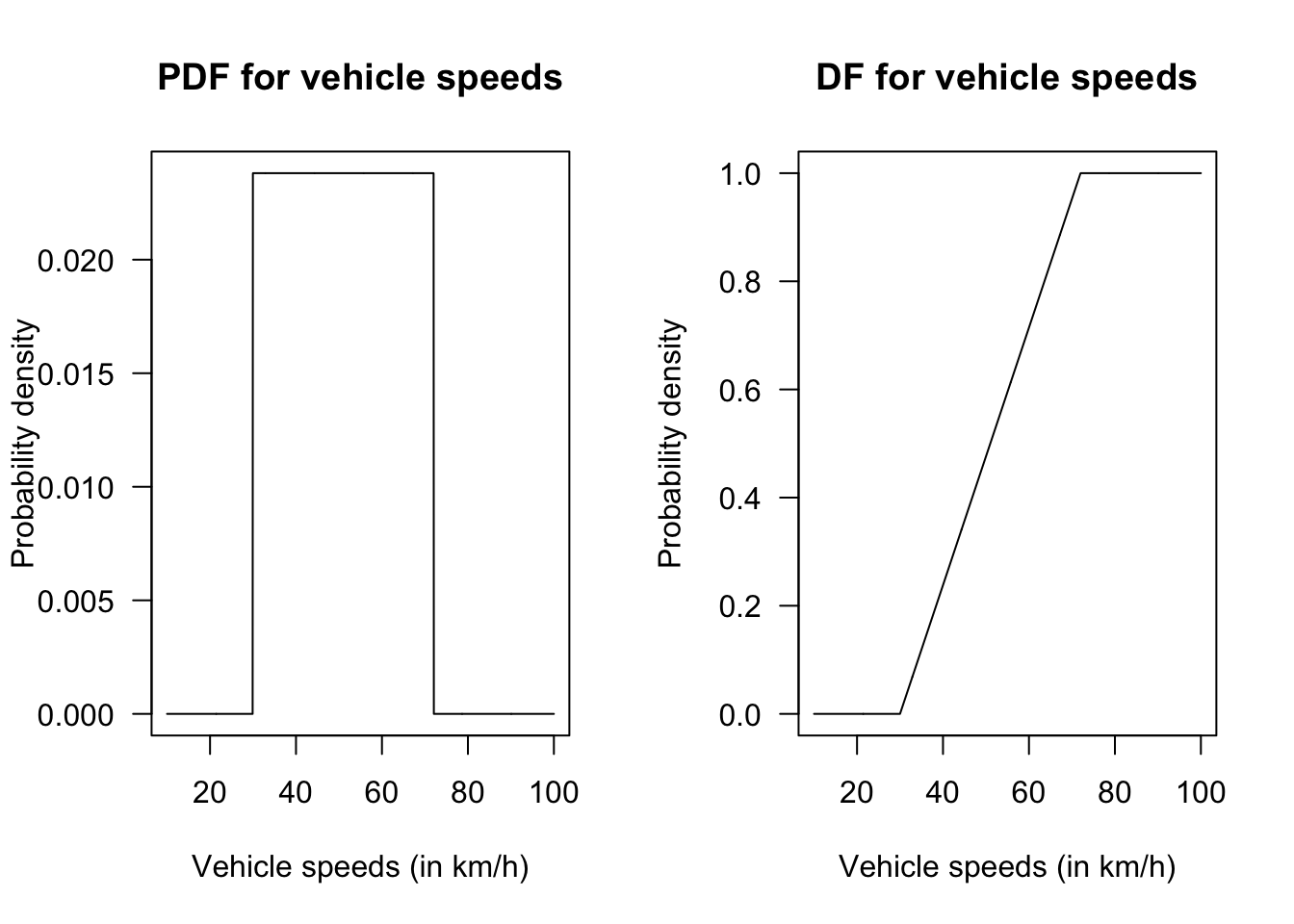

FIGURE F.43: Vehicle speeds.

Exercise 7.21.

About $2.4$% of vehicles are excluded.
$Y$ has the distribution of $X \mid (X > 30 \cap X < 72)$ if $X \sim N(48, 8.8^2)$. The PDF is \[ f_Y(y) = \frac{1}{8.8k \sqrt{2\pi}} \exp\left\{ -\frac{1}{2}\left( \frac{y - 48}{8.8}\right)^2 \right\} \qquad\text{for $30\le y \le 72$}; \] where $k \approx \Phi(-2.045455) + (1 - \Phi(2.727273)) = 0.02359804$.

# Proportion excluded:
pnorm(30, 48, 8.8) + # Slower than 30
   (1 - pnorm(72, 48, 8.8)) # Faster than 72
#> [1] 0.02359804

Exercise 7.24.

See Fig. F.44.
$\operatorname{E}[X] = \alpha \beta \approx 38.4$ and $\operatorname{var}[X] = \alpha \beta^2 \approx 54.54$, so standard deviation is about $7.38$.
$\Pr(C > 30 \mid C < 50) = \Pr(30 < C < 50) / \Pr(C < 50)\approx 0.870$.

alpha <- 27.05; beta <- 1.42

x <- seq(0, 80, length = 200)

par(mfrow = c(1, 2))

plot( y = dgamma(x, shape = alpha, scale = beta),
      x = x,
      las = 1, lwd = 3, type = "l",
      xlab = expression(italic(x)),
      ylab = "Prob. fn")
plot( y = pgamma(x, shape = alpha, scale = beta),
      x = x,
      type = "l", las = 1, lwd = 3,
      xlab = expression(italic(x)),
      ylab = "Dist. fn")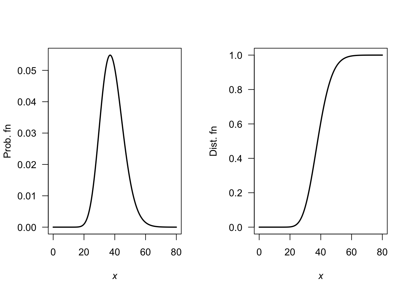

FIGURE F.44: The gamma distribution for the concrete diffusion model.


( pgamma(50, shape = alpha, scale = beta) - 
  pgamma(30, shape = alpha, scale = beta) ) /
pgamma(50, shape = alpha, scale = beta)
#> [1] 0.8701039

Exercise 7.25.

See Fig. F.45.
About $0.0228$.
About $2.17$ kg/m^$3$.
About $2.21$ kg/m^$3$.

mn <- 2; sd <- 0.2

x <- seq(1.2, 2.8, length = 200)

par(mfrow = c(1, 2))
plot( y = dnorm(x, mean = mn, sd = sd),
      x = x,
      xlab = expression(italic(x)),
      ylab = "Prob. fn",
      type = "l", lwd = 3)
plot( y = pnorm(x, mean = mn, sd = sd ),
      x = x,
      xlab = expression(italic(x)),
      ylab = "Dist. fn",
      type = "l", lwd = 3)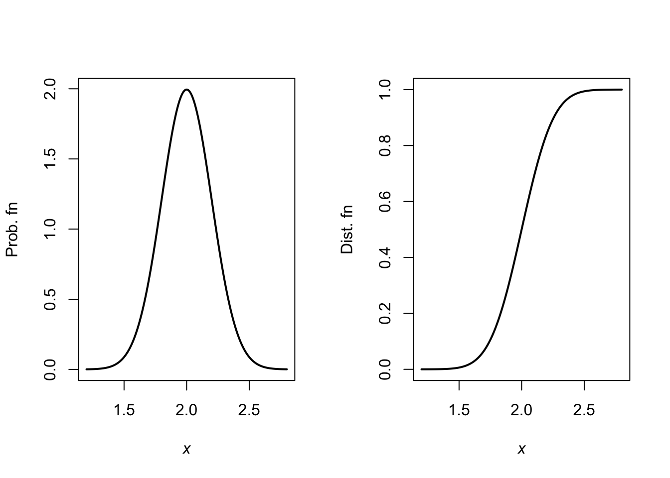

FIGURE F.45: The gamma distribution for the surface chloride concentrations model.


1 - pnorm(2.4, mean = mn, sd = sd)
#> [1] 0.02275013
qnorm(0.8, mean = mn, sd = sd)
#> [1] 2.168324
qnorm(0.85, mean = mn, sd = sd)
#> [1] 2.207287

Exercise 7.26.

See Fig. F.46.
$F_X(x) = \int_0^x ab t^{a - 1} (1 - t^a)^{b - 1} \, dt = 1 - (1 - x^a)^b$.
With $b = 1$, the PDF is $p_X(x) = a x^{a - 1}$. Also, \[ \text{Beta}(a, 1) = \frac{x^{a - 1} (1 - x)^1 - 1}{B(a, 1)} = \frac{x^{a - 1} \Gamma(a + 1)}{\Gamma(a) \, \Gamma(a)} = a x^{a - 1}, \] which is the same as above.
With $a = b = 1$, the PDF is $p_X(x) = 1$, which is the continuous uniform distribution.
Write $Y = 1 - X$; then $p_X(x) = ab(1 - y)^{a - 1} (y^a) ^{b - 1}$.

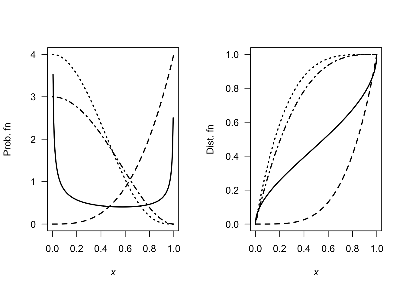
FIGURE F.46: Some Kumaraswamy distributions.

Exercise 7.27. $\text{CV} = \frac{\sqrt{a\beta^2}}{\alpha\beta} = 1/\sqrt{\alpha}$, which is constant.

Exercise 7.28. For the given beta distribution, $\operatorname{E}[V] = 0.287/(0.287 + 0.926) = 0.2366...$ and $\operatorname{var}[V] = 0.08161874$.

$\operatorname{E}[S] = \operatorname{E}[4.5 + 11V] = 4.5 + 11\operatorname{E}[V] = 7.10$ minutes. $\operatorname{var}[S] = 11^2\times\operatorname{var}[V] = 9.875$ minutes².
See Fig. F.47.

v <- seq(0, 1, length = 500)

PDFv <- dbeta(v, shape1 = 0.287, shape2 = 0.926)

plot( PDFv ~ v,
      type = "l", las = 1, lwd = 3,
      xlim = c(0, 1), ylim = c(0, 5),
      xlab = expression(italic(V)),
      ylab = "PDF",
      main = "Distribution of V")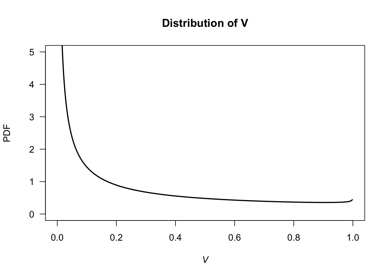

FIGURE F.47: Service times.

Exercise 7.29.

$\operatorname{E}[T] = \operatorname{E}[0.5 + W] = 0.5 + \operatorname{E}[W] = 0.5 + 16.5 = 17.0$.
$\operatorname{var}[T] = \operatorname{var}[0.5 + W] = \operatorname{var}[W] = 16.5^2$, so the std dev is $16.5$.
$\Pr(T > 1) = \Pr( [W + 0.5] > 1 ) = \Pr(W > 0.5) = 0.9702$.

beta <- 16.5
x <- seq(0, 80, length = 1000)

yB <- dexp(x, rate = 1/beta)

plot( yB ~  x,
      type = "l", las = 1, lwd = 3,
      ylim = c(0, 0.06),
      main = expression(PDF~"for"~italic(W)),
      xlab = expression(italic(w)),
      ylab = "Prob. fn.")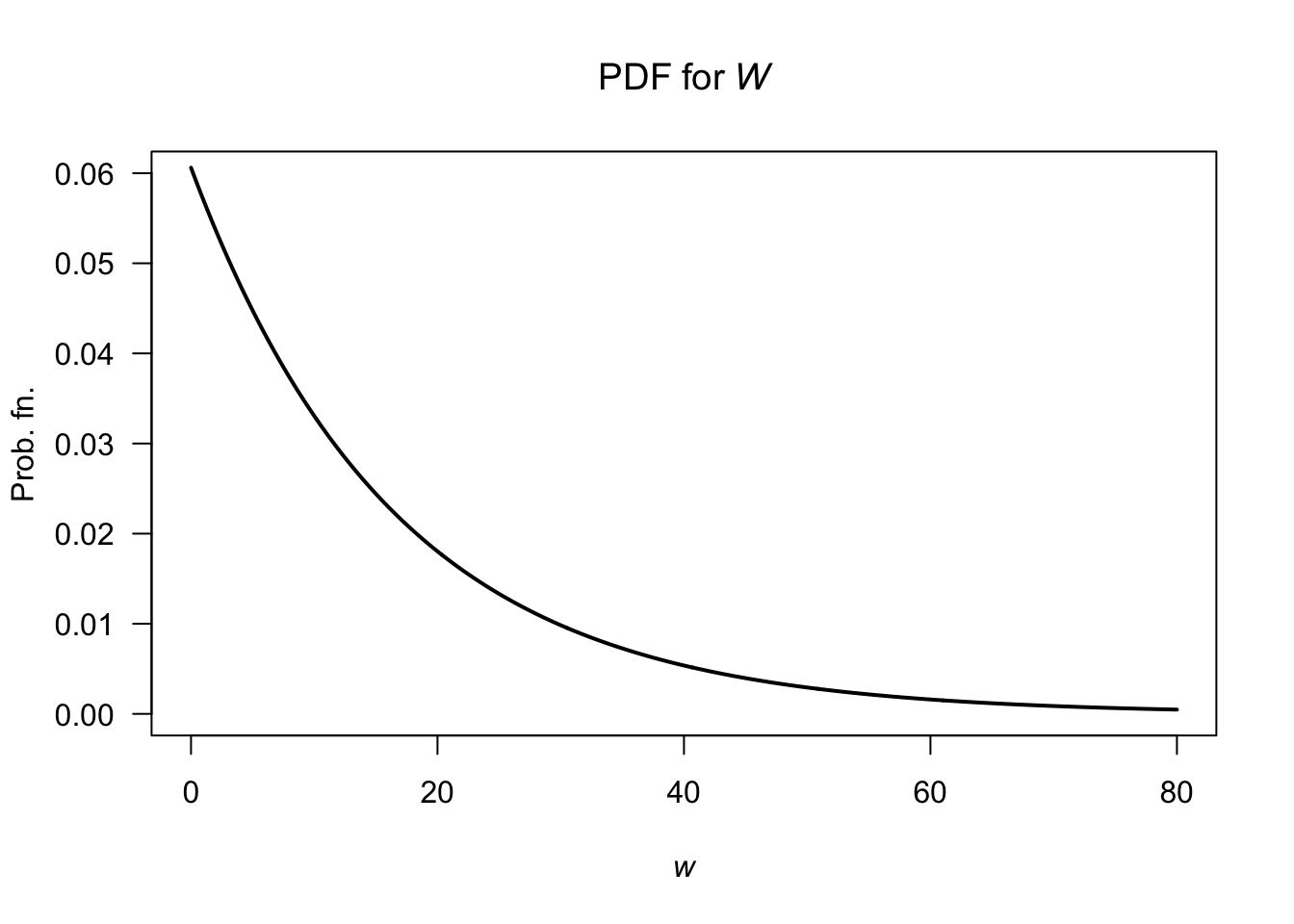

FIGURE F.48: Exponential distribution for hospitals.


# Part 3
1 - pexp(0.5, rate = 1/beta) # 0.9701515
#> [1] 0.9701515

Exercise 7.32.

In summer: If the event lasts more than $1$ hour, what is the probability that it eventually lasts more than three hours?
In winter: If the event lasts more than $1$ hour, what is the probability that it lasts less than two hours?

alpha <- 2; betaS <- 0.04; betaW <- 0.03
x <- seq(0, 1, length = 1000)

yS <- dgamma( x, shape = alpha, scale = betaS)
yW <- dgamma( x, shape = alpha, scale = betaW)

plot( range(c(yS, yW)) ~  range(x),
      type = "n", # No plot, just canvas
      las = 1,
      xlab = "Event duration (in ??)",
      ylab = "Prob. fn.")
lines(yS ~ x, lty = 1, lwd = 3)
lines(yW ~ x, lty = 2, lwd = 3)
legend( "topright",
        lwd = 3, lty = 1:2,
        legend = c("Summer", "Winter"))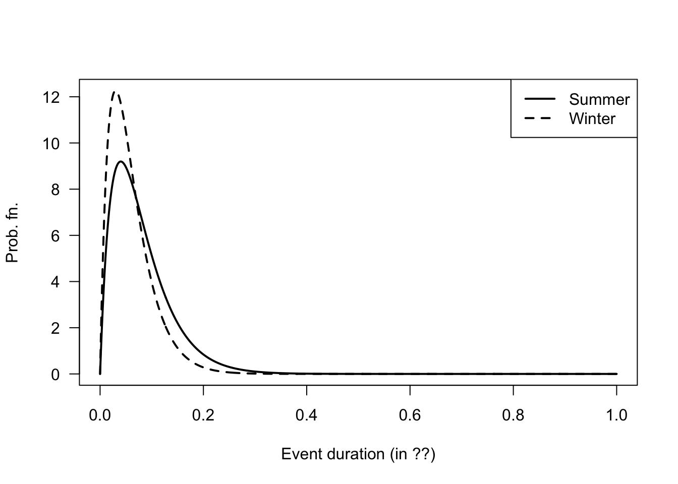

FIGURE F.49: Winter and summer

1 - pgamma(6/24, shape = alpha, scale = betaW)
#> [1] 0.002243448
1 - pgamma(6/24, shape = alpha, scale = betaS)
#> [1] 0.01399579

Exercise 7.34.

$\operatorname{E}[X] = \alpha\beta = 3.76$ days. $\operatorname{var}[X] = \alpha\beta^2 = 12.75$ days², so std dev is $3.571$ days.
The main difference is at the lower end of the distribution.
About $35%$ (gamma) and $31%$ (exponential).
Both just over $10$ days.

alpha <- 1.11; beta <- 3.39

x <- seq(0, 15, length = 500)
yGamma <- dgamma(x, shape = alpha, scale = beta)
yExp <- dexp(x, rate = 1/beta)

plot( range (c(yGamma, yExp)) ~ range(x),
      type = "n", # No plot, just canvas
      las = 1,
      xlab = "Duration of symptoms (in days)",
      ylab = "Prob. fn.")
lines( yGamma ~ x,
       lwd = 2, lty = 1)
lines( yExp ~ x,
       lwd = 2, lty = 2)
legend( "topright",
        lwd = 2, lty = 1:2,
        legend = c("Gamma", "Exponential"))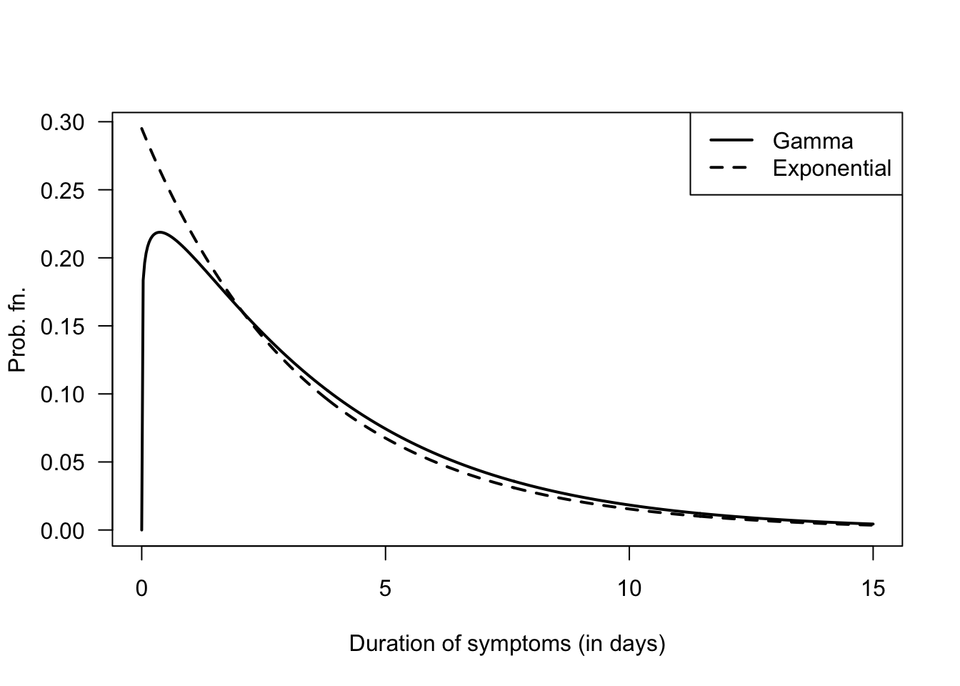

FIGURE F.50: Gamma and exponential


## Part 3
1 - pgamma(4, shape = alpha, scale = beta) # 0.3505492
#> [1] 0.3505492
1 - pexp(4, rate = 1/beta) # 0.3072969
#> [1] 0.3072969

## Part 4
qgamma(0.95, shape = alpha, scale = beta) # 10.86655
#> [1] 10.86655
qexp(0.95, rate = 1/beta) # 10.15553
#> [1] 10.15553

Exercise 7.35.

About $25.2$%.
$\Pr(T > 7 \mid T > 5) = \Pr(T > 7)/\Pr(T > 5)$ or about $33.8$%.
About $7$:$30$pm.

pnorm(5, mean = 6, sd = 1.5)
#> [1] 0.2524925

(1 - pnorm(7, mean = 6, sd = 1.5) ) /
  (1 - pnorm(5, mean = 6, sd = 1.5) )
#> [1] 0.3377793

qnorm(0.85, mean = 6, sd = 1.5)
#> [1] 7.55465

Exercise 7.36. Write $X$ for the percentage of clay content in soil.

For the two counties:

County A:
- $\operatorname{E}[X] = m / (m + n) = 0.708$ or about $70.8$%.
- $\operatorname{var}[X] = 0.01196957$ so the standard deviation is about $10.9$%.
County B:
- $\operatorname{E}[X] = m / (m + n) = 0.513$ or about $51.3$%.
- $\operatorname{var}[X] = 0.02939085$ so the standard deviation is about $17.0$%.

About $96$% for County A; about $53$% for County B. These look reasonable from the plots.

x <- seq(0, 1, length = 1000)
yA <- dbeta(x, shape1 = 11.52, shape2 = 4.75)
yB <- dbeta(x, shape1 = 3.85, shape2 = 3.65)

plot( range( c(yA, yB)) ~ range(100 * x),
      type = "n", #No plot, just canvas
      las = 1,
      xlab = "Percentage clay",
      ylab = "Prob. fn.")
lines( yA ~ I(100 * x),
       lwd = 3, lty = 1)
lines( yB ~ I(100 * x),
       lwd = 3, lty = 2)
legend("top", lty = 1:2, lwd = 3,
       legend = c("Location A", "Location B"))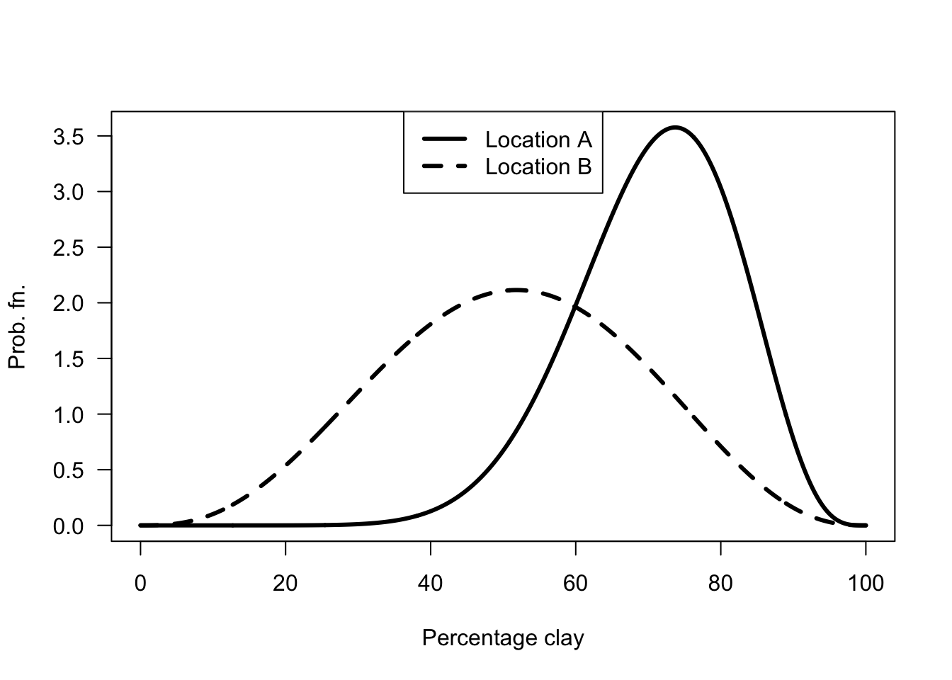

FIGURE F.51: Clay content


## Part 3
qbeta( 0.5, shape1 = 11.52, shape2 = 4.75) #  0.7167495
#> [1] 0.7167495
qbeta( 0.5, shape1 = 3.85,  shape2 = 3.65) # 0.5145787
#> [1] 0.5145787

Exercise 7.38.

Note that if $Y = X - \Delta$, then $Y$ has a gamma distribution, with $\alpha = 2.5$ and $\beta = 0.8$, with $\operatorname{E}[Y] = \alpha\beta = 2$ and $\operatorname{var}[Y] = \alpha\beta^2 = 1.6$.

$\operatorname{E}[X] = \operatorname{E}[Y + \Delta] = 3.2$ seconds. $\operatorname{var}[X] = \operatorname{var}[Y] = 1.6$ seconds^$2$.

numSims <- 1000
yHeadway <- rgamma( n = numSims, shape = 2.5, rate = 0.8)
xHeadway <- yHeadway + 1.2
hist(xHeadway,
     las = 1, lwd = 2,
     xlim = c(0, max(xHeadway)),
     main = "Histogram of headway",
     ylab = "Prob. fn.",
     xlab = "Headway (in sec)")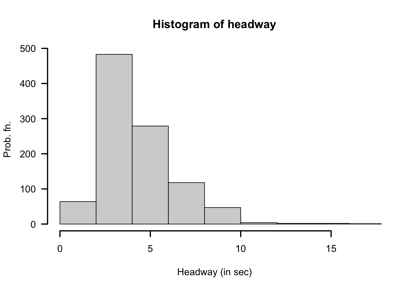

FIGURE F.52: Headways


xMean <- 3.2; xVar <- 1.6
xLo <- 3.2 - 2 * sqrt(xVar)
xHi <- 3.2 + 2 * sqrt(xVar)
cat("Limits", xLo, "and", xHi, "\n")
#> Limits 0.6701779 and 5.729822

# Part 3
Num <- sum( (xHeadway < xHi ) & (xHeadway > xLo) )
EmpiricalProp <- Num / numSims
EmpiricalProp
#> [1] 0.798

# Part 4: Tchebyshev: AT LEAST this proportion
k <- 2
1 - 1/k^2
#> [1] 0.75

Exercise 7.41.

htMean <- function(x) {
  7.5 * x + 70
}
htSD <- function(x) {
  0.4575 * x + 1.515
}

NumSims <- 10000

Ages <- c(
  rep(2, NumSims * 0.32),
  rep(3, NumSims * 0.33),
  rep(4, NumSims * 0.25),
  rep(5, NumSims * 0.10)
)

Hts <- rnorm(NumSims,
             mean = htMean(Ages),
             sd = htSD(Ages))
hist(Hts,
     las = 1,
     xlab = "Heights (in cm)")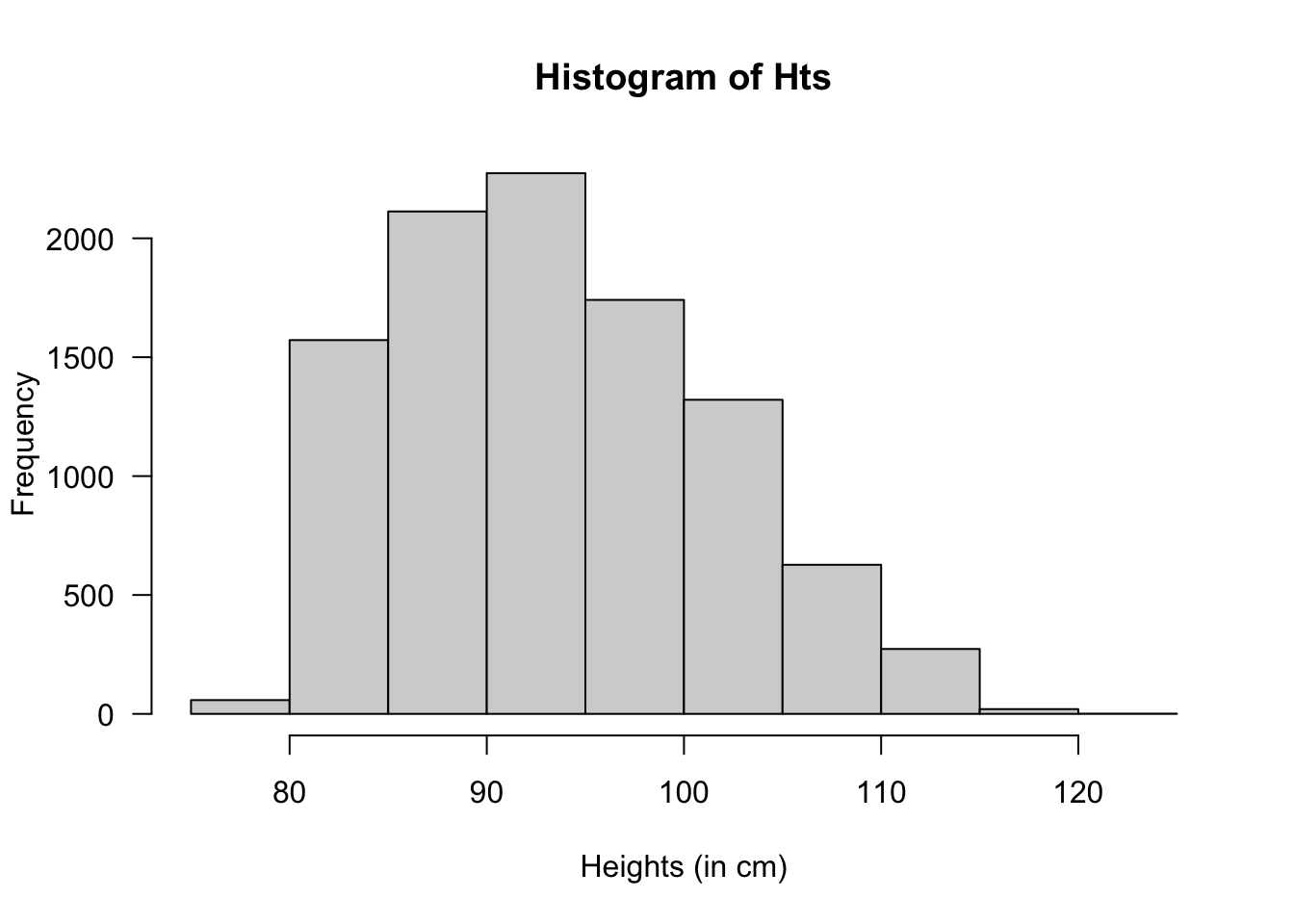

FIGURE F.53: Heights of children at day-care facilities


# Taller than 100:
cat("Taller than 100cm:", sum( Hts > 100) / NumSims * 100, "%\n")
#> Taller than 100cm: 22.41 %
# Mean and variance:
cat("Mean:", mean( Hts ), "cm; ",
    "Std dev: ", sd(Hts), "cm\n")
#> Mean: 93.50605 cm;  Std dev:  7.961026 cm

# Sort the heights to find where the tallest 20% are:
cat("Tallest 15% are taller than", 
    sort(Hts)[ NumSims * 0.85], "cm\n")
#> Tallest 15% are taller than 102.5178 cm

Exercise 7.42. Normal: $\operatorname{var}[X] = \sigma^2 \mu^0$, so $\phi = \sigma^2$ and $p = 0$.
Poisson: $\operatorname{var}[X] = \mu$, so $\phi = 1$ and $p = 1$.
Gamma: $\operatorname{var}[X] = \phi \mu^2$, so $\phi = ???$ and $p = 2$.

Exercise 7.44. The triangle with points $A$, $B$ and the centre $C$ of the circle has sides of length $1$, $1$ and $\sqrt{3}$ respectively. Using the cosine rule, the $\angle ACB = 120^\circ$, in degrees. The probability is $120/360 = 1/3$.

Exercise 7.45. TBA.

Exercise 7.22. TBA.

Exercise 7.23. $f_X(x) = \lambda \exp(-\lambda x)$ for $x > 0$ and $\lambda > 0$; hence $f'_X(x) = -\lambda^2 \exp(-\lambda x) < 0$ for all $x > 0$.

Exercise 7.46.

$\Pr(T_A < 240)$: pnorm(240, mean = 250, sd = 36), or about $0.3901$.
$\Pr(T_B < 240)$: pnorm(240, mean = 280, sd = 36), or about $0.1333$.
Since independent: pnorm(240,250,36) * pnorm(240,280,36) or about $0.0521$.
Since independent: (1-pnorm(240,250,36)) * (1-pnorm(240,280,36)) or about $0.5282$.
pnorm(300,250,36) - pnorm(240,250,36), or about $0.5270$.
The distribution looks normally distributed.

# Parts 6 to 9
num_sims <- 10000
TA <- rnorm(num_sims, mean = 250, sd = 36)
TB <- rnorm(num_sims, mean = 280, sd = 36)
T_difference <- TB - TA
cat("P(Runner A finishes first):", sum(TA < TB)/num_sims, "\n")
#> P(Runner A finishes first): 0.7193
cat("P(Runner A finishes 30 mins faster):", sum( (TA+30) < TB)/num_sims, "\n")
#> P(Runner A finishes 30 mins faster): 0.4932
cat("Mean time diff:", mean(T_difference), "\n")
#> Mean time diff: 29.37893
cat("SD time diff:", sd(T_difference), "\n")
#> SD time diff: 50.71436
hist(T_difference, freq = FALSE, las = 1,
     xlab = "Difference between times")

Exercise 7.47.

Lifter $A$: mean_A <- exp(5.20 + 0.12^2/2), or about $182.58\,\text{kg}$.
Lifter $B$: mean_B <- exp(5.10 + 0.12^2/2), or about $165.15\,\text{kg}$.
1 - plnorm(190, meanlog = 5.20, sdlog = 0.12), or about $0.3476$.
1 - plnorm(190, meanlog = 5.10, sdlog = 0.12), or about $0.110$.
(1 - plnorm(190, 5.20, 0.12)) * (1 - plnorm(190, 5.10, 0.12)) or about $0.0383$.
plnorm(190, 5.20, 0.12) * plnorm(190, 5.10, 0.12) or about $0.5805$.
plnorm(210, 5.20, 0.12) - plnorm(180, 5.20, 0.12), or about $0.4133$.

# Parts 7 to 10
num_sims <- 10000
WA <- rlnorm(num_sims, meanlog = 5.20, sdlog = 0.12)
WB <- rlnorm(num_sims, meanlog = 5.10, sdlog = 0.12)
W_difference <- WA - WB

cat("P(Lifter A lifts more):", mean(WA > WB), "\n")
#> P(Lifter A lifts more): 0.7233
cat("P(Lifter A lifts at least 10 kg more):", mean(WA >= WB + 10), "\n")
#> P(Lifter A lifts at least 10 kg more): 0.5914
cat("Mean lifting difference:", mean(W_difference), "\n")
#> Mean lifting difference: 17.2035
cat("SD lifting difference:", sd(W_difference), "\n")
#> SD lifting difference: 28.99874
hist(W_difference, las = 1, freq = FALSE,
     main = "Estimated PDF of W_A - W_B",
     xlab = "Difference in lifting weight (kg)")

Exercise 7.47.

\[ f_X(x) = \begin{cases} 2(x - a)/\big( (b - a)(c - a)\big) & \text{for $a\le x \le b$};\\ 2(c - x)/\big( (c - b)(c - a)\big) & \text{for $b < x \le c$}; \end{cases} \] and \[ F_X(x) = \begin{cases} 0 & \text{for $x < a$};\\ (x - a)^2/\big( (b - a)(c - a)\big) & \text{for $a\le x \le b$};\\ 1 - (c - x)^2/\big( (c - b)(c - a)\big) & \text{for $b < x \le c$};\\ 1 & \text{for $x > c$}. \end{cases} \]

F.7 Answers for Chap. 8

Exercise 8.1.

Continuous: can take any positive real value.
$S_X = (0, \infty)$.
$Y = X$ when $x \le 50$; $Y = 50$ when $X > 50$.
$S_Y = [0, 50]$.
$Y$ is mixed random; a point mass at $y = 50$.
See Fig. F.54 (left).
$F_Y(y) = 0$ for $y < 0$; $F_Y(y) = 1 - \exp(-y/20)$ for $0 \le y < 50$; $F_Y(y) = 1$ for $y \ge 50$.
See Fig. F.54 (right).
$\Pr(X > 50) \approx 0.0821$ using the exponential distribution.

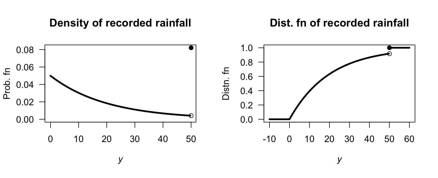
FIGURE F.54: Monthly rainfall recording.

Exercise 8.2.

$X$ is continuous: can take any positive value.
$S_x = (0, \infty)$.
$R = 0$ if $X < 0.1$; $R = X$ if $0.1 \le X \le 70$; $r = 70$ if $X > 70$.
$S_R = \{0\}\cup [0.1, 70]$.
Mixed: point masses at $R=)$ and $R = 70$.
See Fig. F.55 (left).
$F_R(r) = 0$ for $r < 0$; $F_R(r) = 1 - \exp(-0.1/40)$ for $0 \le r < 0.1$; $F_R(r) = 1 - \exp(-r/40)$ for $0.1 < r < 70$; $F_R(r) = 1$ for $r\ge 0$.
See Fig. F.55 (right).
$\Pr(X > 70) \approx 0.174$.
$\Pr(R = 0) = \Pr(X < 0.25) \approx 0.0062$.

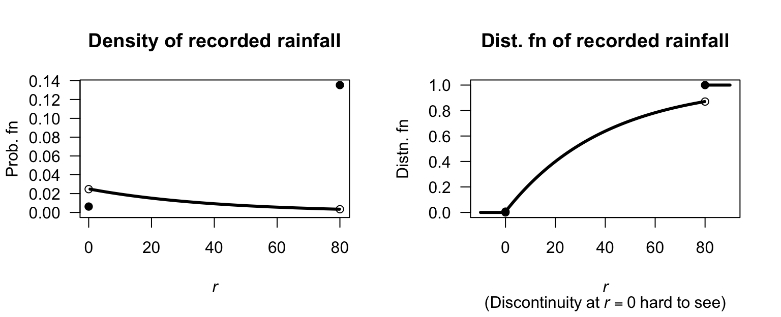
FIGURE F.55: Monthly rainfall recording.

Exercise 8.3.

$F_X(x) = 0$ for $x < 0$; $F_X(x) = 0.4$ for $x = 0$; $F_X(x) = 0.6 + 0.4 \times (1 - \exp(-x/3))$ for $x > 0$.
$S_X(x) = 1$ for $x < 0$; $F_X(x) = 0.6$ for $x = 0$; $F_X(x) = \exp(-x/3)$ for $x > 0$.
TBA

DF1 <- function(x) {
  out <- numeric(length(x))
  out[x == 0] <- 0.4
  out[x > 0] <- 0.4 + 0.6 * (1 - exp(-x[x > 0]/3))
  out
}
1 - DF1(1.5)
#> [1] 0.3639184
DF1(2)
#> [1] 0.6919497
DF1(5) - DF1(1)
#> [1] 0.3165934
uniroot(function(x){DF1(x) - 0.95}, lower = 0, upper = 100)$root
#> [1] 7.454719

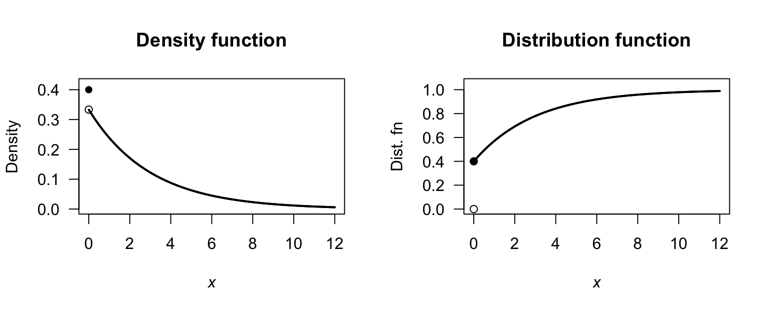
FIGURE F.56: Insurance: exponential.

Exercise 8.4.

$F_X(x) = 0$ for $x < 0$; $F_X(x) = 0.1$ for $x = 0$; $F_X(x) = 0.1 + 0.9 \times (1 - \exp(-x/85))$ for $x > 0$.
$S_X(x) = 1$ for $x < 0$; $F_X(x) = 0.9$ for $x = 0$; $F_X(x) = \exp(-x/85)$ for $x > 0$.
TBA

DF2 <- function(x) {
  out <- numeric(length(x))
  out[x == 0] <- 0.1
  out[x > 0] <- 0.1 + 0.9 * (1 - exp(-x[x > 0]/85))
  out
}
DF2(60)
#> [1] 0.5556945
1 - DF2(50)
#> [1] 0.4997757
DF2(70) - DF2(20)
#> [1] 0.3163126
uniroot(function(x){DF2(x) - 0.25}, lower = 0, upper = 100)$root
#> [1] 15.49735

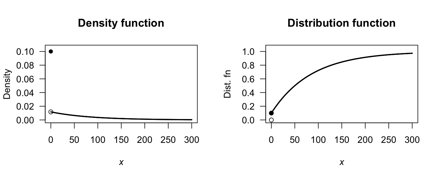
FIGURE F.57: Rainfall; exponential.

Exercise 8.5.

$F_X(x) = 0$ for $x < 0$; $F_X(x) = 0.4$ for $x = 0$; $F_X(x) = ???$ for $x > 0$.
$S_X(x) = 1$ for $x < 0$; $F_X(x) = 0.6$ for $x = 0$; $F_X(x) = ???$ for $x > 0$.
TBA

DF1 <- function(x) {
  out <- numeric(length(x))
  out[x == 0] <- 0.4
  out[x > 0] <- 0.4 + 0.6 * pgamma(x[x > 0], shape = 0.75, scale = 2)
  out
}
1 - DF1(1.5)
#> [1] 0.2090445
DF1(2)
#> [1] 0.843988
DF1(5) - DF1(1)
#> [1] 0.253556
uniroot(function(x){DF1(x) - 0.95}, lower = 0, upper = 100)$root
#> [1] 4.037474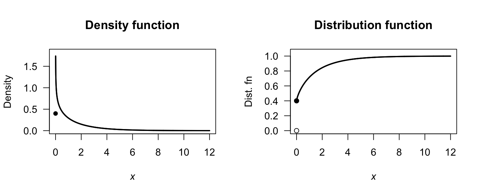

FIGURE F.58: Insurance; gamma.

Exercise 8.6.

$F_X(x) = 0$ for $x < 0$; $F_X(x) = 0.1$ for $x = 0$; $F_X(x) = ???$ for $x > 0$.
$S_X(x) = 1$ for $x < 0$; $F_X(x) = 0.9$ for $x = 0$; $F_X(x) = ???$ for $x > 0$.
TBA.

DF2 <- function(x) {
  out <- numeric(length(x))
  out[x == 0] <- 0.1
  out[x > 0] <- 0.1 + 0.9 * pgamma(x, shape = 0.8, scale = 80)
  out
}
DF2(60)
#> [1] 0.6635868
1 - DF2(50)
#> [1] 0.3888545
DF2(70) - DF2(20)
#> [1] 0.3223154
uniroot(function(x){DF2(x) - 0.25}, lower = 0, upper = 100)$root
#> [1] 8.249703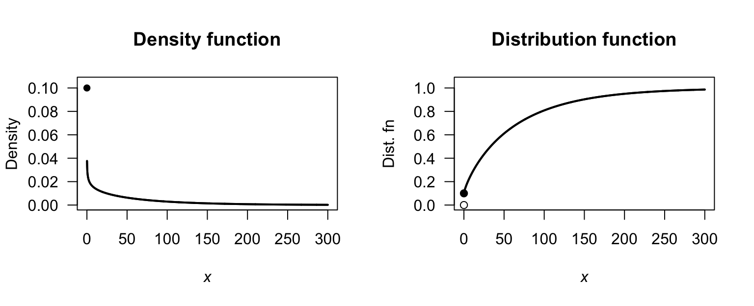

FIGURE F.59: Rainfall; gamma.

Exercise 8.7.

$F_X(x) = 0$ for $x < 0$; $F_X(x) = 0.4$ for $x = 0$; $F_X(x) = ???$ for $x > 0$.
$S_X(x) = 1$ for $x < 0$; $F_X(x) = 0.6$ for $x = 0$; $F_X(x) = ???$ for $x > 0$.
TBA

DF1 <- function(x) {
  out <- numeric(length(x))
  out[x == 0] <- 0.4
  out[x > 0] <- 0.4 + 0.6 * plnorm(x[x > 0], meanlog = 0.75, sdlog = 0.7)
  out
}
1 - DF1(1.5)
#> [1] 0.4132251
DF1(2)
#> [1] 0.6805805
DF1(5) - DF1(1)
#> [1] 0.4489468
uniroot(function(x){DF1(x) - 0.95}, lower = 0, upper = 100)$root
#> [1] 5.573918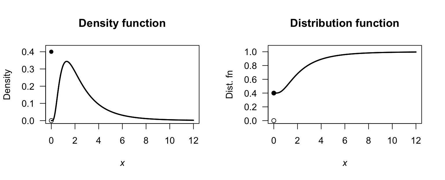

FIGURE F.60: Insurance; log normal

Exercise 8.8.

$F_X(x) = 0$ for $x < 0$; $F_X(x) = 0.1$ for $x = 0$; $F_X(x) = ???$ for $x > 0$.
$S_X(x) = 1$ for $x < 0$; $F_X(x) = 0.9$ for $x = 0$; $F_X(x) = ???$ for $x > 0$.
TBA

DF2 <- function(x) {
  out <- numeric(length(x))
  out[x == 0] <- 0.1
  out[x > 0] <- 0.1 + 0.9 * pgamma(x, shape = 0.8, scale = 80)
  out
}
DF2(60)
#> [1] 0.6635868
1 - DF2(50)
#> [1] 0.3888545
DF2(70) - DF2(20)
#> [1] 0.3223154
uniroot(function(x){DF2(x) - 0.25}, lower = 0, upper = 100)$root
#> [1] 8.249703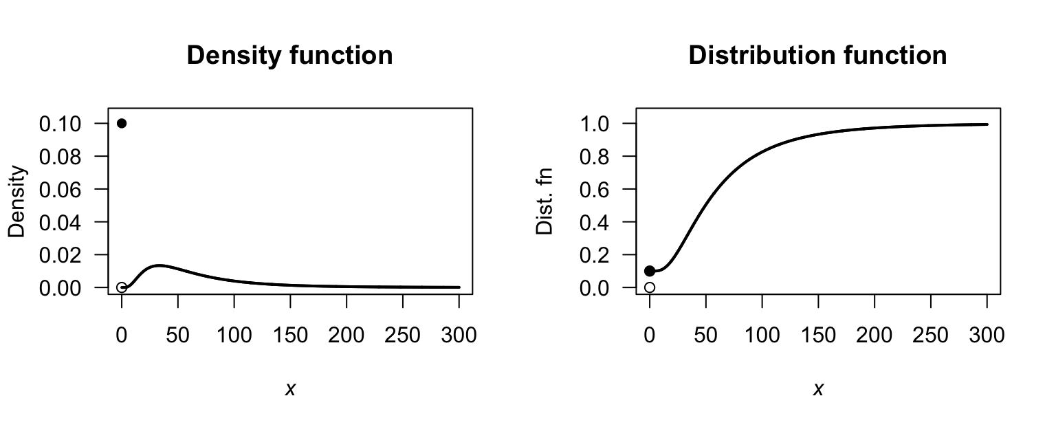

FIGURE F.61: Rainfall; log normal

Exercise 8.9.

$\mu = 4\,200$; $\phi \approx 483$; $\xi = 4/3$.
Mean: $$4\,200$; stand deviation: $\sqrt{33\,600\,000} = \$5\,797$.
$\Pr(T = 0) = \exp(-\lambda) \approx 0.4966$.

See Fig. F.62.

cost_mu <- 4200
cost_phi <- 483 
cost_xi <- 4/3
tweedie_plot(seq(0.01, 30000, length=100), 
             type = "pdf",
             xi=cost_xi, phi=cost_phi, mu=cost_mu)
tweedie_plot(seq(0.01, 30000, length=100), 
             type = "cdf",
             plot_args = list(ylim = c(0, 1)),
             xi=cost_xi, phi=cost_phi, mu=cost_mu)
1 - ptweedie(5000, xi=cost_xi, phi=cost_phi, mu=cost_mu)
#> [1] 0.3285294
ptweedie(20000, xi=cost_xi, phi=cost_phi, mu=cost_mu)
#> [1] 0.9773117
ptweedie(15000, xi=cost_xi, phi=cost_phi, mu=cost_mu) - 
  ptweedie(10000, xi=cost_xi, phi=cost_phi, mu=cost_mu)
#> [1] 0.08626915
qtweedie(0.3, xi=cost_xi, phi=cost_phi, mu=cost_mu)
#> [1] 0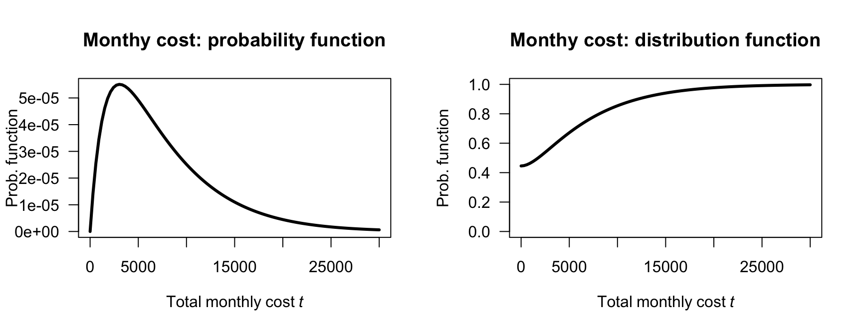

FIGURE F.62: The total monthly cost for a rare procedure.

Exercise 8.10.

$\mu = 160\,000$; $\phi \approx 0.95$; $\xi = 1.25$.
Mean: $$160\,000$; stand deviation: $$20\,000$.
Approximate normal distribution.

See Fig. F.63.

library(tweedie)
cost_mu <- 160000; cost_phi <- 0.95; cost_xi <- 1.25
tweedie_plot(seq(150000, 170000, length = 100), 
             type = "pdf",
             xi = cost_xi, phi = cost_phi, mu = cost_mu)
tweedie_plot(seq(150000, 170000, length = 100), 
             type = "pdf",
             xi = cost_xi, phi = cost_phi, mu = cost_mu)
1 - ptweedie(155000, xi=cost_xi, phi=cost_phi, mu = cost_mu)
#> [1] 0.9980389
ptweedie(165000, xi = cost_xi, phi = cost_phi, mu = cost_mu)
#> [1] 0.9978246
ptweedie(160000, xi = cost_xi, phi = cost_phi, mu = cost_mu) - 
  ptweedie(158000, xi = cost_xi, phi = cost_phi, mu = cost_mu)
#> [1] 0.3753808
qtweedie(0.6, xi = cost_xi, phi = cost_phi, mu = cost_mu)
#> [1] 160438
#
cost_sd <- sqrt( cost_phi * cost_mu^cost_xi)
1 - pnorm(155000, mean = cost_mu, sd = cost_sd )
#> [1] 0.9979326
pnorm(165000, mean = cost_mu, sd = cost_sd )
#> [1] 0.9979326
pnorm(160000, mean = cost_mu, sd = cost_sd ) - 
  pnorm(158000, mean = cost_mu, sd = cost_sd )
#> [1] 0.3743254
qnorm(0.6, mean = cost_mu, sd = cost_sd )
#> [1] 160441.7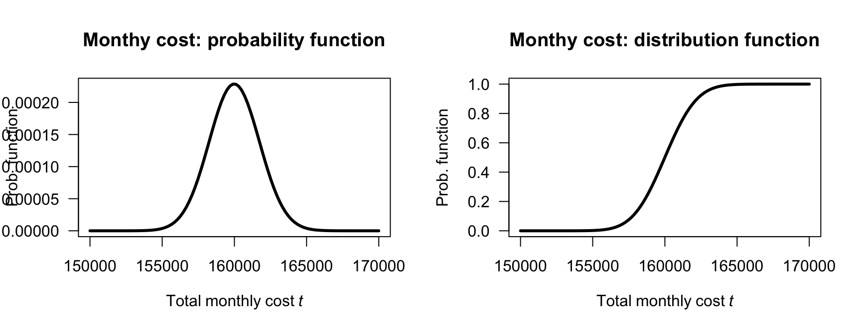

FIGURE F.63: The total monthly cost for a new test procedure.

Exercise 8.11.

Three free parameters. Zero-modified gamma: $p$, $\alpha$, $\beta$; Compound Poisson–gamma: $\lambda$, $\alpha$, $\beta$.
CP-G has mass $\exp(-\lambda)$ at zero, and the positive part is an infinite sum of gamma distributions. ZMG places mass $p$ at zero and the positive part is exactly $\text{Gamma}(\alpha, \beta)$. To match, need $p = \exp(-\lambda)$. But the conditional distribution $S \mid S > 0$ in the CP-G is not a simple Gamma; it is an infinite sum $\sum_{k=1}^\infty w_k \,\text{Gamma}(k\alpha,\beta)$. So the two models produce identical distributions only in degenerate/limiting cases, but not in general.

Exercise 8.12. Overdispersion requires $\operatorname{var}[Y] \ge \operatorname{E}[Y]$.

For ZME: let $\mu^+ = 1/\lambda_e$ (mean of exponential), $p = \Pr(Y = 0)$. So, $\operatorname{E}[Y] = (1 - p)\mu^+, \qquad \operatorname{E}[Y^2] = (1 - p)\cdot 2/\lambda_e^2$. Thus, $\operatorname{var}[Y] = E[Y^2] - (E[Y])^2 = (1 - p)\frac{2}{\lambda_e^2} - (1 - p)^2\frac{1}{\lambda_e^2}$. And so, $\operatorname{var}[Y] = \frac{(1 - p)(1 + p)}{\lambda_e^2}$.

For overdispersion: $\frac{(1 - p)(1 + p)}{\lambda_e^2} > \frac{(1-p)}{\lambda_e}$, hence $\frac{1 + p}{\lambda_e} > 1 \Rightarrow \lambda_e < 1 + p$, so overdispersion. This holds whenever $\operatorname{E}[Y] > 0$ and $p > 0$ combined with a large enough mean, confirming overdispersion in practical settings.

For CP-G: $\operatorname{E}[S] = \lambda \alpha/\beta$, $\operatorname{var}[S] = \lambda \alpha (\alpha + 1)/\beta^2$ and $\operatorname{var}[S] \ge \operatorname{E}[S]$ so that $\lambda\alpha(\alpha + 1)/\beta^2 \ge \lambda\alpha/\beta$ and hence $(\alpha + 1)/\beta > 1$.

This holds when $\alpha + 1 > \beta$, which covers a wide range of practical parameters. When $\operatorname{E}[S] > 0$ (i.e. $\lambda > 0$), we always have $\operatorname{var}[S]/E[S] = (\alpha + 1)/\beta > 0$, and typically $> 1$.

Exercise 8.13. Fix $\operatorname{E}[S] = \mu$, so $\lambda \cdot \alpha/\beta = \mu$, and hold $\alpha/\beta = \mu/\lambda$ constant as $\lambda \to \infty$.

The cumulant generating function of $S$ is: \[ K_S(t) = \lambda\left[\left(\frac{\beta}{\beta - t}\right)^\alpha - 1\right]. \] As $\lambda \to \infty$ with $\alpha = \mu\beta/\lambda \to 0$, using $\log(1 + x) \approx x$ for small $\alpha$: \[\begin{align*} & \left(\frac{\beta}{\beta-t}\right)^\alpha - 1 \approx \alpha \log\frac{\beta}{\beta - t}\\ \Rightarrow & K_S(t) \approx \lambda \cdot \frac{\mu\beta}{\lambda} \log\frac{\beta}{\beta - t}\\ = &\mu\beta \log\frac{\beta}{\beta-t} \end{align*}\] This is the CGF of a Gamma$(\mu\beta,\, \beta)$ distribution (i.e., mean $\mu$, shape $\mu\beta$).

As $\lambda \to \infty$ with mean fixed, the CP-G converges to a Gamma distribution; the zero mass vanishes and the distribution becomes continuous.

Exercise 8.14.

Total probability: \[ \Pr(Y = 0) + \int_0^\infty 0.6\,e^{-y}\,dy = 0.4 + 0.6\left[-e^{-y}\right]_0^\infty = 0.4 + 0.6(1) = 1. \]
Find \[ F_Y(y) = \begin{cases} 0 & \text{for $y < 0$};\\ 0.4 & \text{for $y = 0$};\\ 0.4 + 0.6(1 - \exp(-y)) & \text{for $y > 0$}. \end{cases} \]
$\Pr(Y > 1) = 1 - F_Y(1) = 1 - [0.4 + 0.6(1 - \exp(-1))] = 0.6 \exp(-1) \approx 0.2207$.
$\Pr(0\le Y \le 3) = F_Y(3) - F_Y(0^{-}) = (1 - 0.6\exp(-3)) - 0 \approx 0.9701$. Note: We use $F(0^{-}) = 0$ and not $F(0)$ since the interval includes $Y = 0$, which already has probability mass $0.4$ included.

Exercise 8.15.

$\Pr(X > 0) = 1 - \Pr(X = 0) = 1 - 0.75 = 0.25$.
For a gamma, $\mu_c = \alpha\beta$; $\operatorname{E}[X] = (1 - p)\mu_c = 0.75 \times (2\times 1) = 1.5$.
For a gamma, $\sigma_c^2 = \alpha\beta^2$; $\operatorname{var}[X] = (1 - p)\sigma_c^2 + p(1 - p)\mu_c^2 = 4.6875$.
$P(X>3)$ is $0.25$ times the gamma probability that $X>3$: 0.25 * (1 - pgamma(3, shape = 2, scale = 1)), or about $0.0498$.

Exercise 8.16. Care: $p = \Pr(X = 0) = 0.4$.

For a gamma, $\mu_c = \alpha\beta$; $\operatorname{E}[X] = (1 - p)\mu_c = 0.6 \times (3\times 2) = 3.6\,\text{kg}$.
For a gamma, $\sigma_c^2 = \alpha\beta^2$; $\operatorname{var}[X] = (1 - p)\sigma_c^2 + p(1 - p)\mu_c^2 = 5.44\,\text{kg}^2$.
$P(X>5)$ is $0.6$ times the gamma probability that $X>5$: 0.6 * (1 - pgamma(5, shape = 3, scale = 2)), or about $0.326$.
pgamma(0.2, shape = 3, scale = 2), or about $3.1\,\text{kg}$.

Exercise 8.17.

n_sim <- 1000
lambda <- 0.5; alpha <- 2; beta_rate <- 1

S <- sapply(1:n_sim, function(i) {
  N <- rpois(1, 
             lambda)
  if (N == 0) return(0)
  sum(rgamma(N, shape = alpha, rate = beta_rate))
})

cat("E[S] theoretical:", lambda * alpha / beta_rate, "\n")
#> E[S] theoretical: 1
cat("E[S] simulated:  ", mean(S), "\n")
#> E[S] simulated:   1.014859
cat("Var(S) theoretical:", lambda * alpha * (alpha + 1) / beta_rate^2, "\n")
#> Var(S) theoretical: 3
cat("Var(S) simulated:  ", var(S), "\n")
#> Var(S) simulated:   3.18858
cat("Pr(S = 0) theoretical:", exp(-lambda), "\n")
#> Pr(S = 0) theoretical: 0.6065307
cat("Pr(S = 0) simulated:  ", mean(S == 0), "\n")
#> Pr(S = 0) simulated:   0.603

hist(S[S > 0], 
     breaks = 40, las = 1,
     main = "Total claim amount S | S > 0", 
     xlab = "S ($)", 
     ylab = "Count")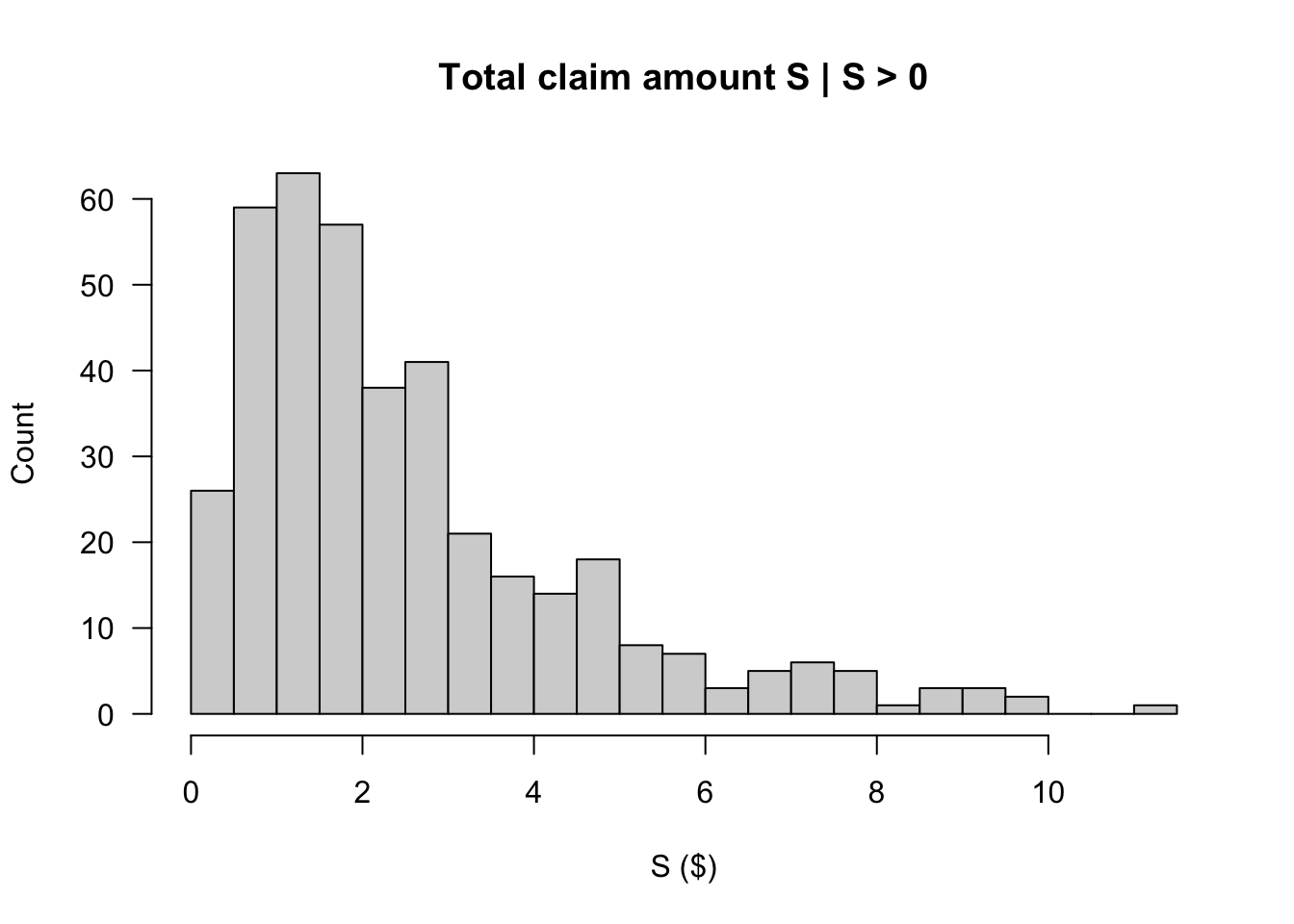

Exercise 8.18.

$\Pr(Y = 0) = \Pr(N = 0) = \exp(-2) = 0.1353$; about $13.5$%.
For a gamma distribution, $\operatorname{E}[X] = \alpha\beta = 2$; about $2$ million dollars per fire.
We have $\operatorname{E}[X] = \lambda\alpha\beta = 4$; about $4$ million dollars per month.
$\operatorname{E}[Y] = \lambda\alpha\beta/(1 - \exp(-\lambda)) = 4.62$; about $4.62$ million dollars per month.
See below; about $5.4$ millon dollars.

lambda_fire <- 2; alpha_fire <- 1; beta_fire <- 2

## 1. Pr(S = 0)
cat("Pr(zero fire damage):", exp(-lambda_fire), "\n")
#> Pr(zero fire damage): 0.1353353

## 2. Mean damage given S > 0
n_sim <- 50000
S_fire <- sapply(1:n_sim, function(i) {
  N <- rpois(1, lambda_fire)
  if (N == 0) return(0)
  sum(rgamma(N, shape = alpha_fire, 
             rate = 1/beta_fire))  # rate parameterisation
})

cat("Mean damage | number fires > 1:", mean(S_fire[S_fire > 1]), "\n")
#> Mean damage | number fires > 1: 5.375251
cat("Theoretical E[S]:", lambda_fire * alpha_fire * beta_fire, "\n")
#> Theoretical E[S]: 4

Exercise 8.19.

Matching mean and proportion of zeros. Let ZM have $p_0$, $\mu^+ = \operatorname{E}[Y \mid Y>0]$, and CP-G have $\lambda$, $\alpha$, $\beta$. Set $p_0 = \exp(-\lambda)$ (same zero probability) and $(1 - p_0)\mu^+ = \lambda\alpha/\beta$ (same mean). This gives us one equation relating parameters: infinitely many solutions exist, so yes, we can always find such parameters.
If $\lambda = 1$, $\alpha = 2$, $\beta = 1$ for CP-G, then $\Pr(S = 0) = \exp(-1) \approx 0.368$, $\operatorname{E}[S] = 2$. For the ZM, set $p_0 = \exp(-1)$, $\mu^+ = \operatorname{E}[S]/(1 - p_0) = 2/(1 - \exp(-1) \approx 3.164$. So, use $\text{Gamma}(\alpha^+=2, \beta^+ = 2/\mu^+)$ for ZM positive part.
Variance comparison:

lambda_c <- 1; alpha_c <- 2; beta_c <- 1

p0 <- exp(-lambda_c)
ES <- lambda_c * alpha_c / beta_c  # = 2
mu_plus <- ES / (1 - p0)

# ZM variance
alpha_zm <- 2
beta_zm <- alpha_zm / mu_plus
var_plus <- alpha_zm / beta_zm^2
E_plus2 <- var_plus + mu_plus^2
var_ZM <- (1 - p0) * E_plus2 - ES^2

# CPG variance
var_CPG <- lambda_c * alpha_c * (alpha_c + 1) / beta_c^2

cat("ZM  variance:", round(var_ZM, 4), "\n")
#> ZM  variance: 5.4919
cat("CPG variance:", round(var_CPG, 4), "\n")
#> CPG variance: 6

Simulation verification

n_sim <- 2000

# CP-G simulation
S_cpg <- sapply(1:n_sim, function(i) {
  N <- rpois(1, lambda_c)
  if (N == 0) return(0)
  sum(rgamma(N, shape = alpha_c, rate = beta_c))
})

# ZM simulation
S_zm <- ifelse(runif(n_sim) < p0, 0,
               rgamma(n_sim, shape = alpha_zm, rate = beta_zm))

cat("CPG - mean:", round(mean(S_cpg),3), "var:", round(var(S_cpg),3),
    "Pr(0):", round(mean(S_cpg==0),3), "\n")
#> CPG - mean: 2.014 var: 5.934 Pr(0): 0.352
cat("ZM  - mean:", round(mean(S_zm),3),  "var:", round(var(S_zm),3),
    "Pr(0):", round(mean(S_zm==0),3), "\n")
#> ZM  - mean: 1.938 var: 5.289 Pr(0): 0.37

Exercise 8.20.

For the zero-modified distribution with $\Pr(Y = 0) = p$ and $Y\mid Y>0 \sim F^+$: \[ F_Y(y) = \begin{cases} p & \text{for $y = 0$}; \\ p + (1 - p) F^+(y) & \text{for $y > 0$}. \end{cases} \] Inverting: for $\tau \leq p$, $Q_Y(\tau) = 0$. For $\tau > p$: \[ \tau = p + (1 - p)F^+(y) \Rightarrow F^+(y) = \frac{\tau - p}{1 - p}. \] So: \[ Q_Y(\tau) = \begin{cases} 0 & \tau \leq p \\ F^+\!\left(\dfrac{\tau - p}{1 - p}\right) & \tau > p \end{cases} \] where $Q^+$ is the quantile function of the positive part.

Median when $p > 0.5$: since $0.5 < p$, then $Q_Y(0.5) = 0$. The median is $0$.

Exercise 8.21.

p  <- 0.4
sh <- 3    # shape
rt <- 2    # rate  (mean of Gamma = shape/rate = 1.5)

mu_plus    <- sh / rt
var_plus   <- sh / rt^2

# 1. E[Y]
EY <- (1 - p) * mu_plus
cat("E[Y] =", EY, "\n")
#> E[Y] = 0.9

# 2. Var(Y)
# Var(Y) = (1-p)(var+ + mu+^2) - [(1-p)mu+]^2
VarY <- (1 - p) * (var_plus + mu_plus^2) - EY^2
cat("Var(Y) =", VarY, "\n")
#> Var(Y) = 0.99

# 3. Pr(Y > 2)
# Pr(Y > 2) = (1-p)*Pr(Y+ > 2)  [the zero mass contributes 0]
prob_gt2 <- (1 - p) * pgamma(2, shape = sh, rate = rt, lower.tail = FALSE)
cat("Pr(Y > 2) =", round(prob_gt2, 4), "\n")
#> Pr(Y > 2) = 0.1429

# 4. 90th percentile
tau <- 0.90
if (tau <= p) {
  cat("90th percentile = 0\n")
} else {
  q90 <- qgamma((tau - p) / (1 - p), shape = sh, rate = rt)
  cat("90th percentile =", round(q90, 4), "\n")
}
#> 90th percentile = 2.2813

Exercise 8.22.

Effect of $p$ on zero-modified Gamma$(2, 1)$:

p_vals <- c(0.1, 0.3, 0.6, 0.85)
sh2 <- 2; rt2 <- 1
y_seq <- seq(0.001, 10, length.out = 500)

mom_table <- data.frame(
  p     = p_vals,
  EY    = sapply(p_vals, function(p) (1-p)*sh2/rt2),
  VarY  = sapply(p_vals, function(p) {
    mu_p <- sh2/rt2; vp <- sh2/rt2^2; ey <- (1-p)*mu_p
    (1-p)*(vp + mu_p^2) - ey^2
  })
)
print(round(mom_table, 4))
#>      p  EY VarY
#> 1 0.10 1.8 2.16
#> 2 0.30 1.4 2.24
#> 3 0.60 0.8 1.76
#> 4 0.85 0.3 0.81

ltys <- 1:4
plot(y_seq, (1 - p_vals[1]) * dgamma(y_seq, shape = sh2, rate = rt2),
     type = "l", lwd = 2,
     ylim = c(0, 0.6),
     main = "Zero-modified Gamma(2,1) density for varying p\n(point mass at 0 not shown)",
     xlab = "y", ylab = "f(y)")
for (i in 2:length(p_vals)) {
  lines(y_seq, (1 - p_vals[i]) * dgamma(y_seq, shape = sh2, rate = rt2),
        lty = ltys[i], lwd = 2)
}
legend("topright", legend = paste0("p = ", p_vals),
       lty = ltys, lwd = 2, bty = "n")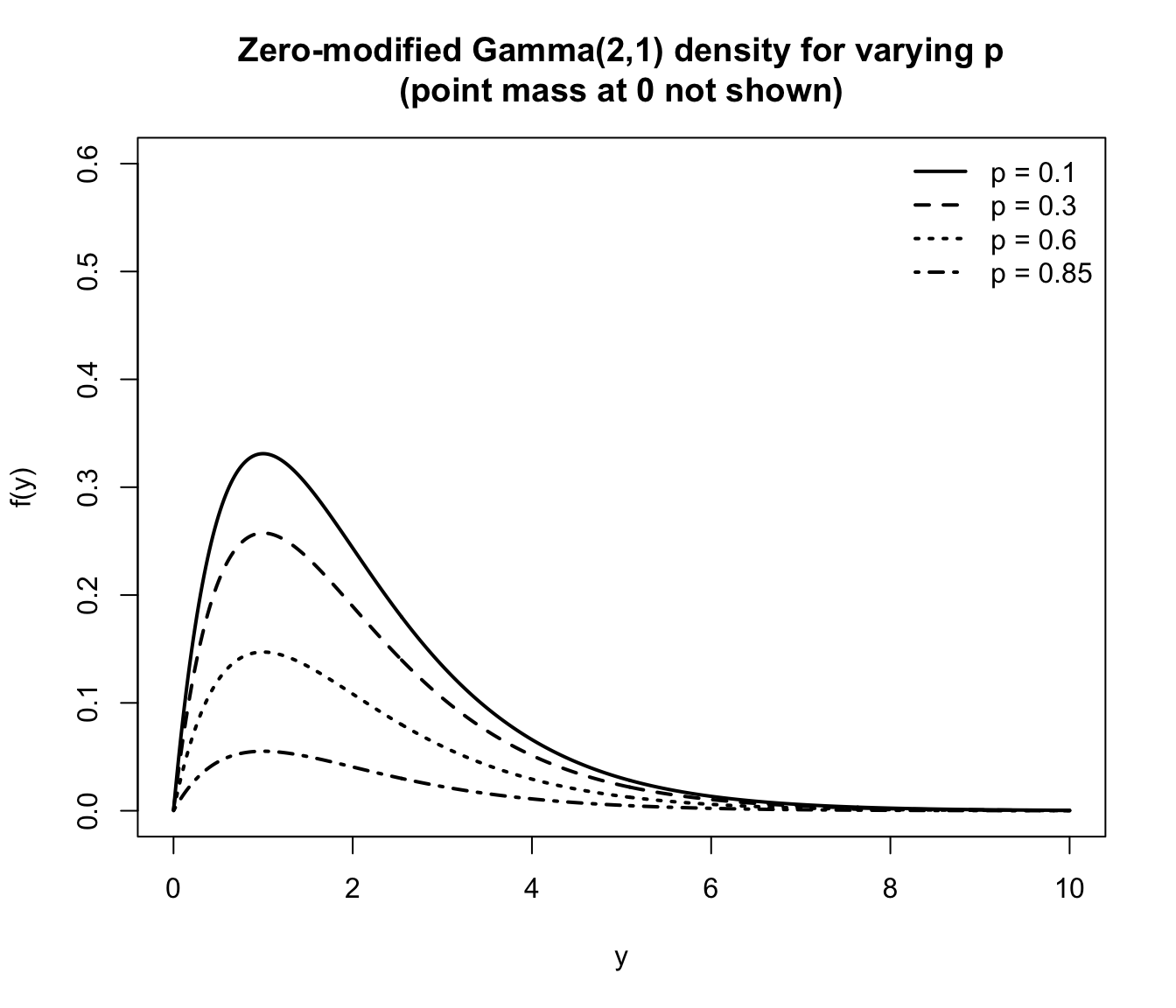

As $p$ increases, the distribution places more mass at zero, shrinking the mean and pulling the continuous part down. The shape of the positive part is unchanged.

Exercise 8.23.

Given: $\Pr(Y = 0) = 0.5$, $\operatorname{E}[Y] = 3$, $\operatorname{var}[Y] = 30$.

p_obs  <- 0.5; EY_obs <- 3; VY_obs <- 30

# E[Y] = (1-p)*mu+  =>  mu+ = E[Y]/(1-p)
mu_plus_hat <- EY_obs / (1 - p_obs)
cat("mu+ =", mu_plus_hat, "\n")
#> mu+ = 6

# Var(Y) = (1-p)(var+ + mu+^2) - E[Y]^2
# => var+ = [Var(Y) + E[Y]^2]/(1-p) - mu+^2
var_plus_hat <- (VY_obs + EY_obs^2) / (1 - p_obs) - mu_plus_hat^2
cat("var+ =", var_plus_hat, "\n")
#> var+ = 42

# Gamma: mu+ = a/b, var+ = a/b^2  =>  b = mu+/var+, a = mu+*b
b_hat <- mu_plus_hat / var_plus_hat
a_hat <- mu_plus_hat * b_hat
cat("Gamma shape (alpha) =", round(a_hat, 4), "\n")
#> Gamma shape (alpha) = 0.8571
cat("Gamma rate  (beta)  =", round(b_hat, 4), "\n")
#> Gamma rate  (beta)  = 0.1429
cat("Is alpha > 0 and beta > 0?", a_hat > 0 && b_hat > 0, "\n")
#> Is alpha > 0 and beta > 0? TRUE

# Plot
y_seq <- seq(0.001, 40, length.out = 600)
dens  <- (1 - p_obs) * dgamma(y_seq, shape = a_hat, rate = b_hat)

plot(y_seq, dens, type = "l", lwd = 2,
     main = "Estimated zero-modified distribution",
     sub  = "Red triangle = point mass at 0",
     xlab = "y", ylab = "density / mass")
segments(x0 = 0, y0 = 0, x1 = 0, y1 = p_obs, 
         lwd = 3, lty = 2)
points(0, p_obs, pch = 17, cex = 1.8)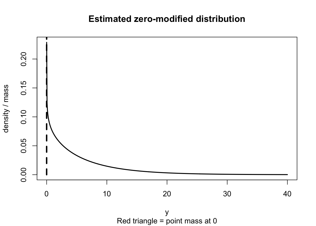

Exercise 8.24.

Link between $\Pr(S = 0)$ and $\operatorname{E}[S]$ In CP-G: $\Pr(S = 0) = \exp(-\lambda)$ and $\operatorname{E}[S] = \lambda\alpha/\beta$. So $\lambda = \beta \operatorname{E}[S]/\alpha$, giving: \[ \Pr(S = 0) = \exp\!\left(-\frac{\beta\,\operatorname{E}[S]}{\alpha}\right). \] There is a direct link: higher mean $\Rightarrow$ smaller $\Pr(S = 0)$.

In the zero-modified model, $p$ and $\operatorname{E}[Y] = (1 - p)\mu^+$ are independently specifiable; no such constraint.

$S \mid S > 0$ is not a simple Gamma: \[ S \mid S > 0 = \sum_{k=1}^N X_k \mid N \geq 1. \]

The conditional distribution of $N \mid N \geq 1$ is a zero-truncated Poisson (not constant), so $S\mid S>0$ is a mixture: \[ f_{S\mid S > 0}(s) = \sum_{k=1}^\infty \Pr(N = k \mid N \geq 1) \cdot f_{\text{Gamma}(k\alpha,\beta)}(s). \] This infinite mixture is not a single Gamma.
Approximate Gamma when $\lambda \to \infty$: As shown in (DIFF EXERCISE), as $\lambda \to \infty$ with fixed mean, $\Pr(S = 0) \to 0$ and $S$ converges to Gamma. So $S\mid S>0 \approx \text{Gamma}$ for large $\lambda$.

Exercise 8.25.

CGF: \[ M_S(t) = \exp\!\left\{\lambda\left[\left(\frac{\beta}{\beta - t}\right)^\alpha - 1\right]\right\}. \] and \[ K_S(t) = \lambda\left[\left(\frac{\beta}{\beta-t}\right)^\alpha - 1\right]. \]
First four cumulants: Differentiating $K_S(t)$ at $t = 0$: \[ \kappa_r = \lambda \cdot \frac{\alpha(\alpha + 1)\cdots(\alpha + r - 1)}{\beta^r} = \lambda \cdot \frac{\Gamma(\alpha + r)}{\Gamma(\alpha)\,\beta^r}. \]

Cumulant	Formula
$\kappa_1 = E[S]$	$\lambda\alpha/\beta$
$\kappa_2 = \text{var}[S]$	$\lambda\alpha(\alpha+1)/\beta^2$
$\kappa_3$	$\lambda\alpha(\alpha+1)(\alpha+2)/\beta^3$
$\kappa_4$	$\lambda\alpha(\alpha+1)(\alpha+2)(\alpha+3)/\beta^4$

Skewness and excess kurtosis \[\begin{align*} \gamma_1 &= \frac{\kappa_3}{\kappa_2^{3/2}} = \frac{\lambda\alpha(\alpha+1)(\alpha+2)/\beta^3}{\left[\lambda\alpha(\alpha+1)/\beta^2\right]^{3/2}}\\ &= \frac{(\alpha+2)}{\sqrt{\lambda\alpha(\alpha+1)}} \cdot \frac{1}{\beta^{1/2}} \cdot \beta = \frac{(\alpha+2)}{\sqrt{\lambda\alpha(\alpha+1)}}\\ \gamma_2 &= \frac{\kappa_4}{\kappa_2^2} = \frac{3(\alpha+2)(\alpha+3)}{\lambda\alpha(\alpha+1)(\alpha+2)} \cdot \frac{(\alpha+1)}{\alpha} \cdot \frac{1}{(\alpha+3)}\cdots \end{align*}\] (simplifies, but positive for all parameters).
Always positively skewed: \[ \gamma_1 = \frac{\alpha + 2}{\sqrt{\lambda\alpha(\alpha + 1)}} > 0. \] since $\alpha > 0$ and $\lambda > 0$.

Exercise 8.26. CP-G with $N \sim \text{Poisson}(3)$, $X_k \sim \text{Gamma}(2, 0.01)$

lambda_e <- 3; alpha_e <- 2; beta_e <- 0.01  # rate parameterisation

# 1. E[S]
ES_e <- lambda_e * alpha_e / beta_e
cat("E[S] =", ES_e, "\n")
#> E[S] = 600

# 2. Var(S)
VarS_e <- lambda_e * alpha_e * (alpha_e + 1) / beta_e^2
cat("Var(S) =", VarS_e, "\n")
#> Var(S) = 180000

# 3. Skewness
gamma1_e <- (alpha_e + 2) / sqrt(lambda_e * alpha_e * (alpha_e + 1))
cat("Skewness gamma1 =", round(gamma1_e, 4), "\n")
#> Skewness gamma1 = 0.9428

# 4. Pr(S = 0)
cat("Pr(S = 0) =", round(exp(-lambda_e), 4), "\n")
#> Pr(S = 0) = 0.0498

# 5. Pr(S > 1000) by simulation
n_sim <- 100000
S_sim <- sapply(1:n_sim, function(i) {
  N <- rpois(1, lambda_e)
  if (N == 0) return(0)
  sum(rgamma(N, shape = alpha_e, rate = beta_e))
})
cat("Pr(S > 1000) approx", round(mean(S_sim > 1000), 4), "\n")
#> Pr(S > 1000) approx 0.1661

Exercise 8.27.

CP-G moment table and density for varying $\lambda$, $\alpha$ (fixed $\beta = 1$).

beta_p <- 1
lambdas <- c(0.5, 2, 8)
alphas  <- c(0.5, 2)

params <- expand.grid(lambda = lambdas, alpha = alphas)
params$ES   <- params$lambda * params$alpha / beta_p
params$VarS <- params$lambda * params$alpha * (params$alpha + 1) / beta_p^2
params$Pr0  <- exp(-params$lambda)
params$skew <- (params$alpha + 2) / sqrt(params$lambda * params$alpha * (params$alpha + 1))

print(round(params, 3))
#>   lambda alpha    ES   VarS   Pr0  skew
#> 1    0.5   0.5  0.25  0.375 0.607 4.082
#> 2    2.0   0.5  1.00  1.500 0.135 2.041
#> 3    8.0   0.5  4.00  6.000 0.000 1.021
#> 4    0.5   2.0  1.00  3.000 0.607 2.309
#> 5    2.0   2.0  4.00 12.000 0.135 1.155
#> 6    8.0   2.0 16.00 48.000 0.000 0.577

n_s <- 20000
par(mfrow = c(3, 2), mar = c(4, 4, 3, 1))
for (i in 1:nrow(params)) {
  lam <- params$lambda[i]; alp <- params$alpha[i]
  S <- sapply(1:n_s, function(j) {
    N <- rpois(1, lam)
    if (N == 0) return(0)
    sum(rgamma(N, shape = alp, rate = beta_p))
  })
  S_pos <- S[S > 0]
  d <- density(S_pos, from = 0)
  plot(d, main = sprintf("lambda=%.1f, alpha=%.1f", lam, alp),
       xlab = "S", ylab = "Density", lwd = 3)
  d$x <- c(0, d$x) # To make polygon work correctly
  d$y <- c(0, d$y)
  polygon(d, col = adjustcolor("grey", alpha.f = 0.3), border = NA)
}

par(mfrow = c(1, 1))

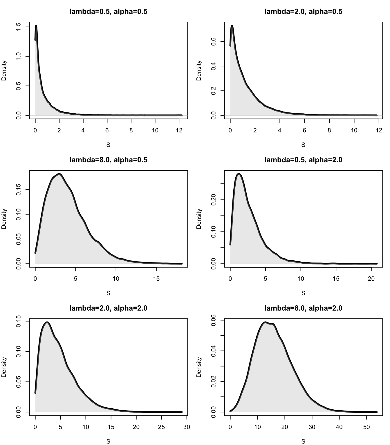
Exercise 8.28.

Tweedie power-variance relationship: For CP-G: $\operatorname{E}[S] = \lambda\alpha/\beta$ and $\operatorname{var}[S] = \lambda\alpha(\alpha + 1)/\beta^2$: \[ \operatorname{var}[S] = \frac{\alpha+1}{\beta} \cdot \frac{\lambda\alpha}{\beta} = \frac{\alpha + 1}{\lambda\alpha/\beta} \cdot \left(\frac{\lambda\alpha}{\beta}\right)^2 \cdot \frac{1}{\lambda\alpha/\beta}. \] More directly, write $\mu = \operatorname{E}[S]$: \[ \operatorname{var}[S] = \frac{(\alpha + 1)}{\beta} \mu = \frac{(\alpha + 1)}{\lambda\alpha}\mu^2 \cdot \frac{\lambda\alpha/\beta}{\mu}. \] After algebra, $\operatorname{var}[S] = \phi\,\mu^p$ where $p = (\alpha + 2)/(\alpha + 1)$.

Show $p \in (1,2)$ for $\alpha > 0$: \[ p = \frac{\alpha + 2}{\alpha + 1} = 1 + \frac{1}{\alpha + 1}. \]

As $\alpha \to 0^+$: $p \to 1 + 1 = 2$.
As $\alpha \to \infty$: $p \to 1$.
Strictly decreasing in $\alpha$, so $p \in (1, 2)$ for all $\alpha > 0$.

# Numerical verification
alphas_tw <- c(0.1, 0.5, 1, 2, 5, 10, 50)
p_tw <- (alphas_tw + 2) / (alphas_tw + 1)
cat("alpha:", alphas_tw, "\n")
#> alpha: 0.1 0.5 1 2 5 10 50
cat("p:    ", round(p_tw, 4), "\n")
#> p:     1.9091 1.6667 1.5 1.3333 1.1667 1.0909 1.0196
cat("All p in (1,2)?", all(p_tw > 1 & p_tw < 2), "\n")
#> All p in (1,2)? TRUE

Exercise 8.29. R function for CP-G random sampling:

rcpg <- function(n, lambda, alpha, beta) {
  sapply(1:n, function(i) {
    N <- rpois(1, lambda)
    if (N == 0) return(0)
    sum(rgamma(N, shape = alpha, rate = beta))
  })
}

# Simulate and verify
lam_r <- 2; alp_r <- 3; bet_r <- 0.5
S_r <- rcpg(1e5, lam_r, alp_r, bet_r)

cat("--- Theoretical vs Simulated ---\n")
#> --- Theoretical vs Simulated ---
cat("E[S]:      theory =", lam_r*alp_r/bet_r,
    "  sim =", round(mean(S_r), 3), "\n")
#> E[S]:      theory = 12   sim = 12.02
cat("Var(S):    theory =", lam_r*alp_r*(alp_r+1)/bet_r^2,
    "  sim =", round(var(S_r), 3), "\n")
#> Var(S):    theory = 96   sim = 96.045
cat("Pr(S=0):   theory =", round(exp(-lam_r), 4),
    "  sim =", round(mean(S_r == 0), 4), "\n")
#> Pr(S=0):   theory = 0.1353   sim = 0.1354

# Skewness

Exercise 8.30.

Probability plots for three CP-G distributions:

configs <- list(
  list(lambda=0.5, alpha=1, beta=1),
  list(lambda=2,   alpha=2, beta=0.5),
  list(lambda=5,   alpha=3, beta=2)
)

par(mfrow = c(3, 1), mar = c(4, 4, 3, 1))
for (cfg in configs) {
  S <- rcpg(8000, cfg$lambda, cfg$alpha, cfg$beta)
  p0  <- mean(S == 0)
  eS  <- mean(S)
  S_pos <- S[S > 0]

  # Spike at 0 + density for positive part
  d <- density(S_pos, from = 0)
  ylim_max <- max(d$y, p0 / diff(range(S_pos)) * 5) * 1.1

  plot(d, main = sprintf("CP-G(lambda=%.1f, alpha=%.1f, beta=%.1f)  |  Pr(S=0)=%.3f, E[S]=%.2f",
                          cfg$lambda, cfg$alpha, cfg$beta, p0, eS),
       xlab = "S", ylab = "Density", xlim = c(0, max(S_pos)), lwd = 2)
  segments(x0 = 0, y0 = 0, x1 = 0, y1 = p0 * 3, lwd = 4, lty = 2)
  points(0, p0 * 3, pch = 19, cex = 1.5)
  legend("topright", legend = c("Continuous part", sprintf("Mass at 0: %.3f", p0)),
         lwd = 2, lty = c(1, 2), bty = "n")
}

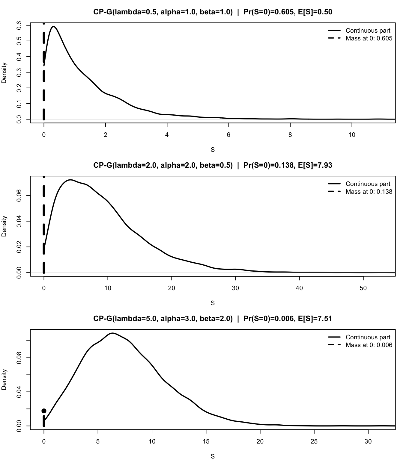
Exercise 8.32.

Matching CP-G and Zero-Modified-Gamma on mean, variance, and $\Pr(X = 0)$:

# CP-G parameters
lam_m <- 2; alp_m <- 2; bet_m <- 1
ES_m   <- lam_m * alp_m / bet_m          # = 4
VarS_m <- lam_m * alp_m*(alp_m+1)/bet_m^2  # = 12
p0_m   <- exp(-lam_m)                    # about 0.135

cat("Target: E[S]=", ES_m, "Var(S)=", VarS_m, "Pr(0)=", round(p0_m,4), "\n")
#> Target: E[S]= 4 Var(S)= 12 Pr(0)= 0.1353

# ZM parameters: match p0, mean, variance
p_zm <- p0_m
mu_plus_zm <- ES_m / (1 - p_zm)
# var_plus from: Var = (1-p)(var+ + mu+^2) - E^2
var_plus_zm <- (VarS_m + ES_m^2)/(1-p_zm) - mu_plus_zm^2

# Gamma parameterisation
bet_zm <- mu_plus_zm / var_plus_zm
alp_zm <- mu_plus_zm * bet_zm
cat("ZM Gamma: shape=", round(alp_zm,4), "rate=", round(bet_zm,4), "\n")
#> ZM Gamma: shape= 1.9487 rate= 0.4212

# Simulate
n_s <- 30000
S_cpg <- rcpg(n_s, lam_m, alp_m, bet_m)
S_zm  <- ifelse(runif(n_s) < p_zm, 0,
                rgamma(n_s, shape = alp_zm, rate = bet_zm))

cat("\nUpper 5% tail:\n")
#> 
#> Upper 5% tail:
cat("CPG P(S > q95):", round(mean(S_cpg > quantile(S_cpg, 0.95)), 4), "\n")
#> CPG P(S > q95): 0.05
cat("ZM  P(S > q95):", round(mean(S_zm  > quantile(S_zm,  0.95)), 4), "\n")
#> ZM  P(S > q95): 0.05

# Density of positive part
d_cpg <- density(S_cpg[S_cpg > 0])
d_zm  <- density(S_zm[S_zm > 0])
xlim  <- c(0, 20)
ylim  <- c(0, max(d_cpg$y, d_zm$y) * 1.1)

plot(d_cpg, col = "grey", lwd = 2, xlim = xlim, ylim = ylim,
     main = "Density of positive part: CP-G vs Zero-Modified Gamma\n(matched on mean, variance, Pr(X=0))",
     xlab = "S", ylab = "Density")
polygon(d_cpg, col = adjustcolor("grey", 0.3), border = NA)
lines(d_zm, col = "coral", lwd = 2)
polygon(d_zm, col = adjustcolor("coral", 0.3), border = NA)
legend("topright", legend = c("CP-G", "Zero-Modified Gamma"),
       col = c("grey", "coral"), lwd = 2, bty = "n")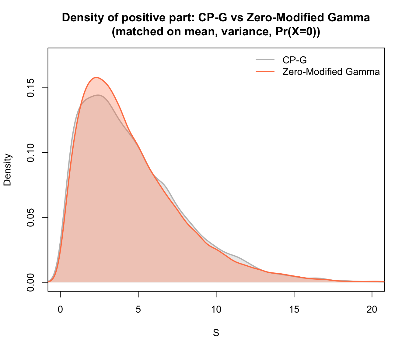

Even with the same mean, variance, and zero probability, the two models differ in the shape of the positive tail. The CP-G tends to have heavier right tails and higher skewness due to the Poisson mixing, while the ZM model has a simpler Gamma positive part. The upper $5$% exceedance probabilities and skewness reveal these differences clearly.

Exercise 8.31. Use the MGFs, the MGF of $T = X_1 + X_2$ is $M_T(t) = M_{X_1}(t) \cdot M_{X_2}(t)$. Substituting the MGFs for the CPG, \[ M_T(t) = \exp\!\left\{(\lambda_1 + \lambda_2)\left[\left(\frac{1}{1-\beta t}\right)^\alpha - 1\right]\right\} \]

This is the MGF of a CPG$(\lambda_1 + \lambda_2, \alpha, \beta)$ distribution. Since the MGF uniquely determines the distribution, $T$ has a CPG$(\lambda_1 + \lambda_2, \alpha, \beta)$.

Reproductive property of CP-G:

n_r <- 50000
S1 <- rcpg(n_r, lambda=2, alpha=1.5, beta=0.5)
S2 <- rcpg(n_r, lambda=3, alpha=1.5, beta=0.5)
T_sum <- S1 + S2  # should behave like CP-G(5, 1.5, 0.5)

lam_T <- 5; alp_T <- 1.5; bet_T <- 0.5

cat("--- T = S1 + S2 vs CP-G(5, 1.5, 0.5) theory ---\n")
#> --- T = S1 + S2 vs CP-G(5, 1.5, 0.5) theory ---
cat("E[T]:    theory =", lam_T*alp_T/bet_T,
    "  sim =", round(mean(T_sum), 3), "\n")
#> E[T]:    theory = 15   sim = 14.91
cat("Var(T):  theory =", lam_T*alp_T*(alp_T+1)/bet_T^2,
    "  sim =", round(var(T_sum), 3), "\n")
#> Var(T):  theory = 75   sim = 73.984
cat("Pr(T=0): theory =", round(exp(-lam_T),4),
    "  sim =", round(mean(T_sum==0), 4), "\n")
#> Pr(T=0): theory = 0.0067   sim = 0.0067

# CDF comparison
x_pts <- quantile(T_sum, probs = seq(0.1, 0.9, 0.1))
T_theory <- rcpg(n_r, lam_T, alp_T, bet_T)
cat("\nCDF comparison at deciles:\n")
#> 
#> CDF comparison at deciles:
df_cdf <- data.frame(
  x      = round(x_pts, 2),
  sim    = round(sapply(x_pts, function(x) mean(T_sum <= x)), 3),
  theory = round(sapply(x_pts, function(x) mean(T_theory <= x)), 3)
)
print(df_cdf)
#>         x sim theory
#> 10%  4.77 0.1  0.098
#> 20%  7.36 0.2  0.196
#> 30%  9.58 0.3  0.297
#> 40% 11.65 0.4  0.397
#> 50% 13.76 0.5  0.498
#> 60% 16.01 0.6  0.598
#> 70% 18.58 0.7  0.698
#> 80% 21.77 0.8  0.799
#> 90% 26.42 0.9  0.896

The CP-G is reproductive: $S_1 + S_2 \sim \text{CP-G}(\lambda_1+\lambda_2, \alpha, \beta)$ when $\alpha$ and $\beta$ are shared.

Exercise 8.33. Consider the CPG distribution.

Hold $\mu = \lambda\alpha\beta$ fixed (so the mean of $X$ is constant) and let $\lambda \to \infty$, $\alpha \to 0$ with $\lambda\alpha$ constant.

The CGF of $X$ is: \[ K_X(t) = \lambda\left[\left(\frac{1}{1-\beta t}\right)^\alpha - 1\right]. \] Write $(1 - \beta t)^{-\alpha} = \exp\{-\alpha \log(1 - \beta t)\}$ and expand for small $\alpha$: \[ (1 - \beta t)^{-\alpha} \approx 1 - \alpha\log(1-\beta t). \] So: \[ K_X(t) \approx \lambda \cdot (-\alpha)\log(1-\beta t) = -(\lambda\alpha)\log(1-\beta t). \] Setting $k = \lambda\alpha$ (which is fixed): \[ K_X(t) \to -k\log(1-\beta t) = \log(1-\beta t)^{-k}. \] This is the CGF (and hence the MGF) of a Gamma$(k, \beta) = \text{Gamma}(\lambda\alpha, \beta)$ distribution.

So as $\lambda \to \infty$ and $\alpha \to 0$ with $\lambda\alpha$ fixed, the CPG distribution converges to a Gamma$(\lambda\alpha, \beta)$ distribution; the point mass at zero vanishes (since $\exp(-\lambda) \to 0$) and the distribution becomes purely continuous. Intuitively, there are so many tiny jumps that the compound sum behaves like a continuous accumulation, converging to a gamma by a law-of-large-numbers argument.

Exercise 8.34. From the law of total expectation, \[ \operatorname{E}[X] = \operatorname{E}[X \mid X = 0] \cdot \Pr(X = 0) + \operatorname{E}[X \mid X > 0] \cdot \Pr(X > 0). \] Then since $\operatorname{E}[X\mid X = 0] = 0$ and $\Pr(X = 0) = \exp(-\lambda)$, \[ \lambda \alpha\beta = 0 + \operatorname{E}[X\mid X>0] \times (1 - \exp(-\lambda)), \] from which we find $\operatorname{E}[X\mid X > 0] = \lambda\alpha\beta/(1 - \exp(-\lambda))$.

F.8 Answers for Chap. 9

Exercise 9.1.

For $0 < x < 2$, the transformation is one-to-one. The inverse transform is $X = Y^{1/3}$, and so $0 < y < 8$.

$F_Y(y) = \Pr(Y\le y) = \Pr(X^3 \le y) = \Pr(X\le y^{1/3}) = F_X( y^{1/3}) = \int_{u = 0}^{y^{1/3}} u/2\,du = \left[u^2/4\right]_{u = 0}^{u = y^{1/3}} = y^{2/3}/4.$ Differentiate to find the PDF: $f_Y(y) = \frac{d}{dy} y^{2/3}/4 = y^{-1/3}/6$.
Since $w(y) = y^{1/3}$, then $w'(y) = y^{-2/3}$. Then: \[\begin{align*} f_Y(y) &= f_X(y) |J|\\ &= y^{1/3}/2 \times \overbrace{y^{-2/3}/3}^{|J|} \\ &= y^{-1/3}/6 \end{align*}\] for $0 < y < 8$.
See Fig. F.64.

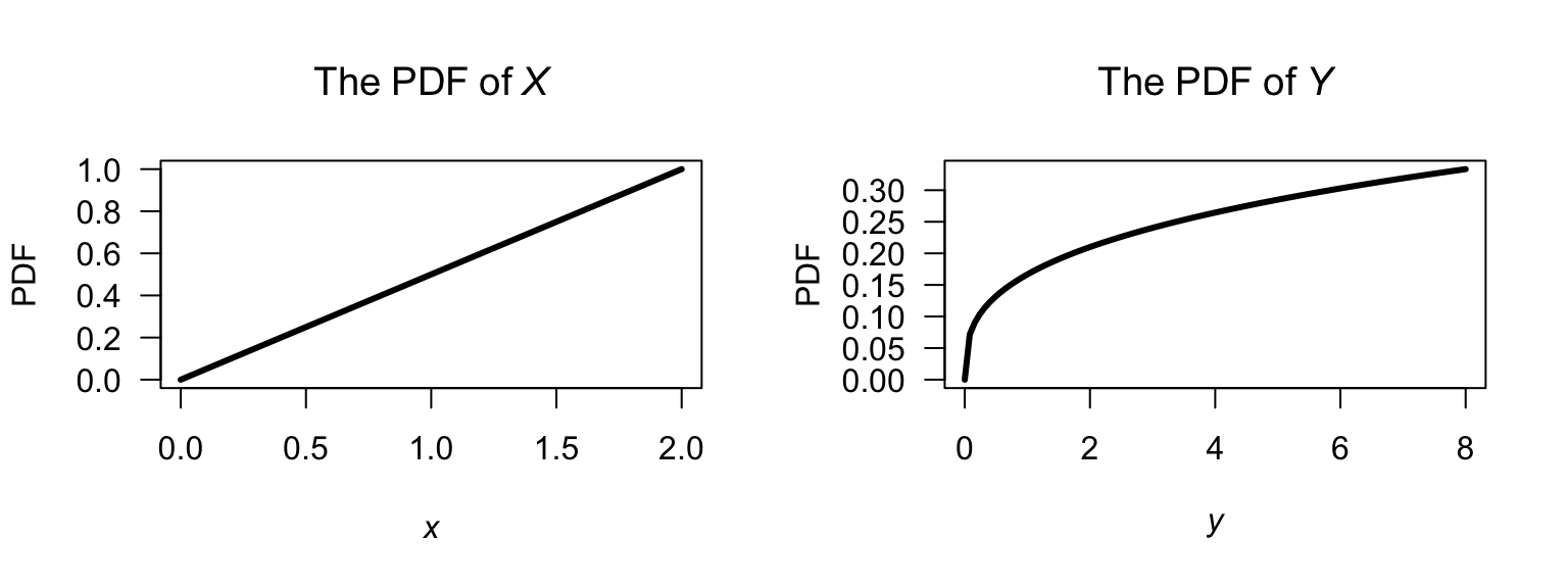
FIGURE F.64: The PDF of $X$ and $Y = X^2$.

Exercise 9.2. For $0 < x < 1$, the transformation is one-to-one. The inverse transform is $Y = \sqrt{X}$, and so $0 < y < 1$. $F_X(x) = 4x/3 - x^3/3$ when $0 < x < 1$.

$F_Y(y) = \Pr(Y\le y) = \Pr(\sqrt{X} \le y) = \Pr(X\le y^2) = F_X( y^2) = 3y^2/2 - y^6/2$. Differentiate to find the PDF: $f_Y(y) = 3y - 3y^5$ for $0 < y < 1$.
Since $w(y) = y^2$, then $w'(y) = 2y$ since $y > 0$. Then: \[\begin{align*} f_Y(y) &= f_X(y) |J|\\ &= 3(1 - y^4)/2 \times 2y = 3y(1 - y^4) \end{align*}\] for $0 < y < 1$.
See Fig. F.65.

$The PDF of $X$ and $Y = \sqrt{X}$.$

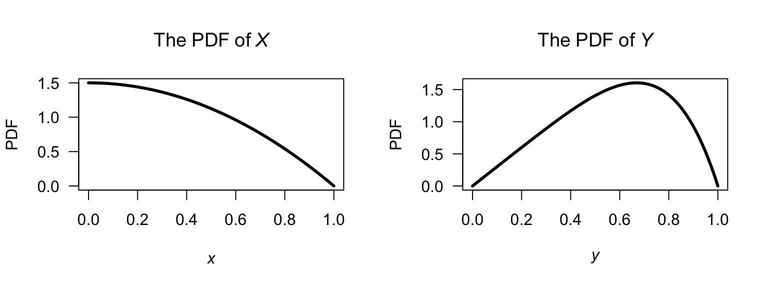
FIGURE F.65: The PDF of $X$ and $Y = \sqrt{X}$.

Exercise 10.22. First:

For $X_1 = 0$, $X_2= 0$ (with prob: $0$): $Y_1 = 0$; $Y_2 = 0$;
For $X_1 = 0$, $X_2= 1$ (with prob. $1/6$): $Y_1 = 1$; $Y_2 = 1$;
For $X_1 = 1$, $X_2= 0$ (with prob. $2/6$): $Y_1 = 1$; $Y_2 = 0$;
For $X_1 = 1$, $X_2= 1$ (with prob. $3/6$): $Y_1 = 2$; $Y_2 = 1$.

Effectively, the first line can be ignored (since the probability is zero), so $Y_1 \in \{1, 2\}$ and $Y_2\in\{0, 1\}$.

From the above, the joint pf is shown in Table F.2.
Hence, from the table: \[ f_{Y_1}(y_1) = \begin{cases} 1/2 & \text{if $y_1 = 1$};\\ 1/2 & \text{if $y_1 = 2$}. \end{cases} \]

TABLE F.2: The joint distribution of $Y_1$ and $Y_2$
	$Y_1 = 1$	$Y_1 = 2$
$Y_2 = 0$	$2/6$	$0$
$Y_2 = 1$	$1/6$	$3/6$

Exercise 9.3. $Y \sim\text{Gamma}(\sum\alpha, \beta)$.

Exercise 9.4. Transformation is not 1-1; and $Y > 0$. Then: \[\begin{align*} F_Y(y) &= \Pr(Y < y)\\ &= \Pr( X^1 < y)\\ &= \Pr( -\sqrt{y} < X < \sqrt{y} ) \quad\text{(draw a diagram!)}\\ &= \int_{-\sqrt{y}}^{\sqrt{y}} \frac{1}{\pi(1 + x^2)}\, dx\\ &= \frac{2}{\pi} \tan^{-1}(\sqrt{y}). \end{align*}\] and so \[ f_Y(y) = \frac{d}{dy} \frac{2}{\pi} \tan^{-1}(\sqrt{y}) = \frac{1}{\pi(y + 1)\sqrt{y}}\quad\text{for $y > 0$}. \]

Exercise 9.5.

Differentiating: $f_X(x) = 1$ for $-1/2 < x < /1/2$}.
First: this transformation is not 1:1 (Fig. F.66). See that $X = \pm\sqrt{4 - Y}$, and that $3.75 < Y < 4$. So, \[\begin{align*} F_Y(y) &= \Pr(Y < y) \\ &= 1 - \Pr( -\sqrt{4 - y} < X < \sqrt{4 - y} )\\ &= 1 - \int_{-\sqrt{4 - y}}^{\sqrt{4 - y}} 1\, dx\\ &= 1 - 2\sqrt{4 - y}, \end{align*}\] and so, differentiating: \[ f_Y(y) = \frac{1}{\sqrt{4 - y}} \quad\text{for $3.75 < Y < 4$} \]

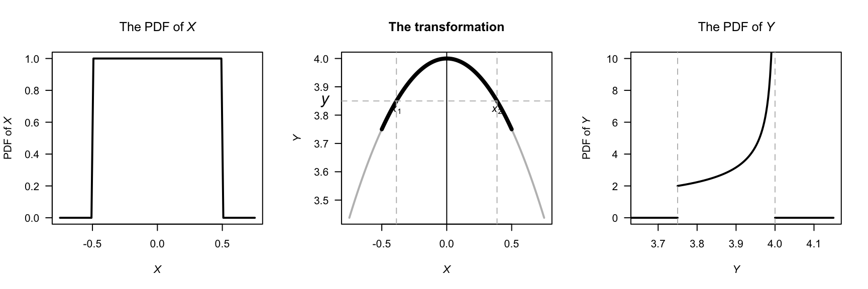
FIGURE F.66: The transformation.

Exercise 9.8.

Given that $f(\theta) = 4/\pi$ for $0 < \theta< \pi/4$, and hence $0 < D < (v^2/g)$. Then: \[\begin{align*} F_D(d) = \Pr(D < d) &= \Pr( v^2/g\sin2\theta < d) \\ &= \Pr(\theta < \frac{1}{2} \sin^{-1}(d g/v^2 ) \\ &= \int_0^{\sin^{-1}(d g/v^2 )/2} \frac{4}{\pi}\, d\theta \\ &= \frac{2}{\pi} \sin^{-1} \left( \frac{dg}{v^2} \right). \end{align*}\] So \[ f_D(d) = \frac{2g}{\pi}\frac{1}{\sqrt{v^4 - d^2 g^2}}\quad\text{for $0 < D < v^2 /g$}. \]

Alternatively: see that $D = v^2\sin 2\theta/g \Rightarrow sin 2\theta = Dg/v^2$, and so \[ \frac{dd}{d\theta} = \frac{2v^2}{g}\cos 2\theta. \] Then, \[\begin{align*} f_D(d) &= \frac{4}{\pi} \left| \frac{g}{2 v^2\cos 2\theta} \right|\\ &= \frac{2g}{\pi v^2 \cos2\theta}\\ &= \frac{2g}{\pi \sqrt{v^4 - d^2 g^2}} \end{align*}\] after (e.g.) drawing the right-angled triangle to re-write $\sin 2\theta = Dg/v^2$. See Fig. F.67.

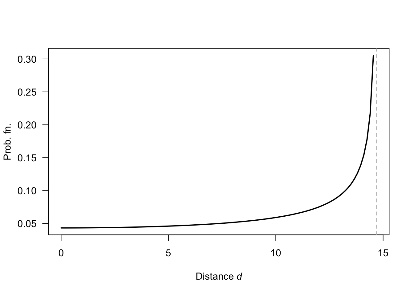
FIGURE F.67: The distance travelled by a projectile.

Exercise 9.9.

$I = 240/R$ and $\log R\sim N(\mu = 10, \sigma^2 = ????)$. Taking logs: $\log I = \log 240 - \log R$. Thus, $\log I \sim N(\log 240 - \mu, \sigma^2)$ and so $I\sim\text{Log-normal}(log 24, 0.1)$.
See Fig. F.68.
$\Pr(I > 30) = \Pr(R < 8)$; since $R$ is log-normal, $\log R\sim N(\log 10, 0.1)$. Thus, $\Pr(R < 8) = \Phi( (\log 8 - \log 10)/\sqrt{0.1}) = \Pr(z < -0.706) \approx 0.24$.
$\operatorname{E}[I] = \exp(\mu + \sigma^2/2)$ for log-normal: $\operatorname{E}[I] = 24\exp(0.05) = 25.23$.
$\operatorname{var}[I] = \exp(\sigma^2 - 1)\exp(2\mu + \sigma^2)$ for log-normal: $\operatorname{E}[I] = 66.9$.
The median current: $24$; reciprocal of mean: $22.85$. Since $1/x$ is non-linear, $\operatorname{E}[1/R] \ne 1/\operatorname{E}]R]$.

FIGURE F.68: The distribution of current in a circuit.

Exercise 9.10. Proceed: \[\begin{align*} F_Y(y) &= \Pr(Y \le y) = \Pr(X \ge \exp(-y/\alpha)) \qquad\text{note the change of direction!}\\ &= \int_{\exp(-y/\alpha)}^1 1\, dx \end{align*}\] so that $f_Y(y) = \frac{1}{\alpha} \exp(-y/\alpha)$ for $y > 0$, which is the exponential distribution.

Exercise 9.11.

$\operatorname{E}[W] = -1/3$; $\operatorname{var}[W] = 17/9\approx 1.8889\dots$.
$\Pr(V = 0) = 1/2$; $\Pr(V = 4) = 1/2$.
Find: \[ F_W(w) = \begin{cases} 0 & \text{for $w < -2$};\\ 1/3 & \text{for $-2 \le w < 0$};\\ 5/6 & \text{for $0 \le w < 2$};\\ 1 & \text{for $w \ge 2$}. \end{cases} \]

Exercise 9.15.

First see that $Y = \log X$. Then: \[\begin{align*} F_Y(y) &= \Pr(Y < y) \\ &= \Pr( \exp X < y)\\ &= \Pr( X < \log y)\\ &= \Phi\left((\log y - \mu)/\sigma\right) \end{align*}\] by the definition of $\Phi(\cdot)$.
Proceed: \[\begin{align*} f_Y(y) &= \frac{d}{dy} \Phi\big((\log y - \mu)/\sigma\big) \\ &= \frac{1}{y} \Phi\big((\log y - \mu)/\sigma\big) \\ &= \frac{1}{y\sqrt{2\pi\sigma^2}} \exp\left[\left( -\frac{ (\log y - \mu)^2}{\sigma}\right)^2\right] \end{align*}\] since the derivative of $\Phi(\cdot)$ (the df of a standard normal distribution) is $\phi(\cdot)$ (the PDF of a standard normal distribution).
See Fig. F.69.
See below: About $0.883$.

par( mfrow = c(2, 2))

x <- seq(0, 8,
         length = 500)

plot( dlnorm(x, meanlog = log(1), sdlog = 1) ~ x,
      xlab = expression(italic(y)),
      ylab = "PDF",
      type = "l",
      main = expression(Log~normal*":"~mu==1~and~sigma==1),
      lwd = 2,
      las = 1)
plot( dlnorm(x, meanlog = log(3), sdlog = 1) ~ x,
      xlab = expression(italic(y)),
      ylab = "PDF",
      type = "l",
      main = expression(Log~normal*":"~mu==3~and~sigma==1),
      lwd = 2,
      las = 1)
plot( dlnorm(x, meanlog = log(1), sdlog = 2) ~ x,
      xlab = expression(italic(y)),
      ylab = "PDF",
      main = expression(Log~normal*":"~mu==1~and~sigma==2),
      type = "l",
      lwd = 2,
      las = 1)
plot( dlnorm(x, meanlog = log(3), sdlog = 2) ~ x,
      xlab = expression(italic(y)),
      ylab = "PDF",
      main = expression(Log~normal*":"~mu==3~and~sigma==2),
      type = "l",
      lwd = 2,
      las = 1)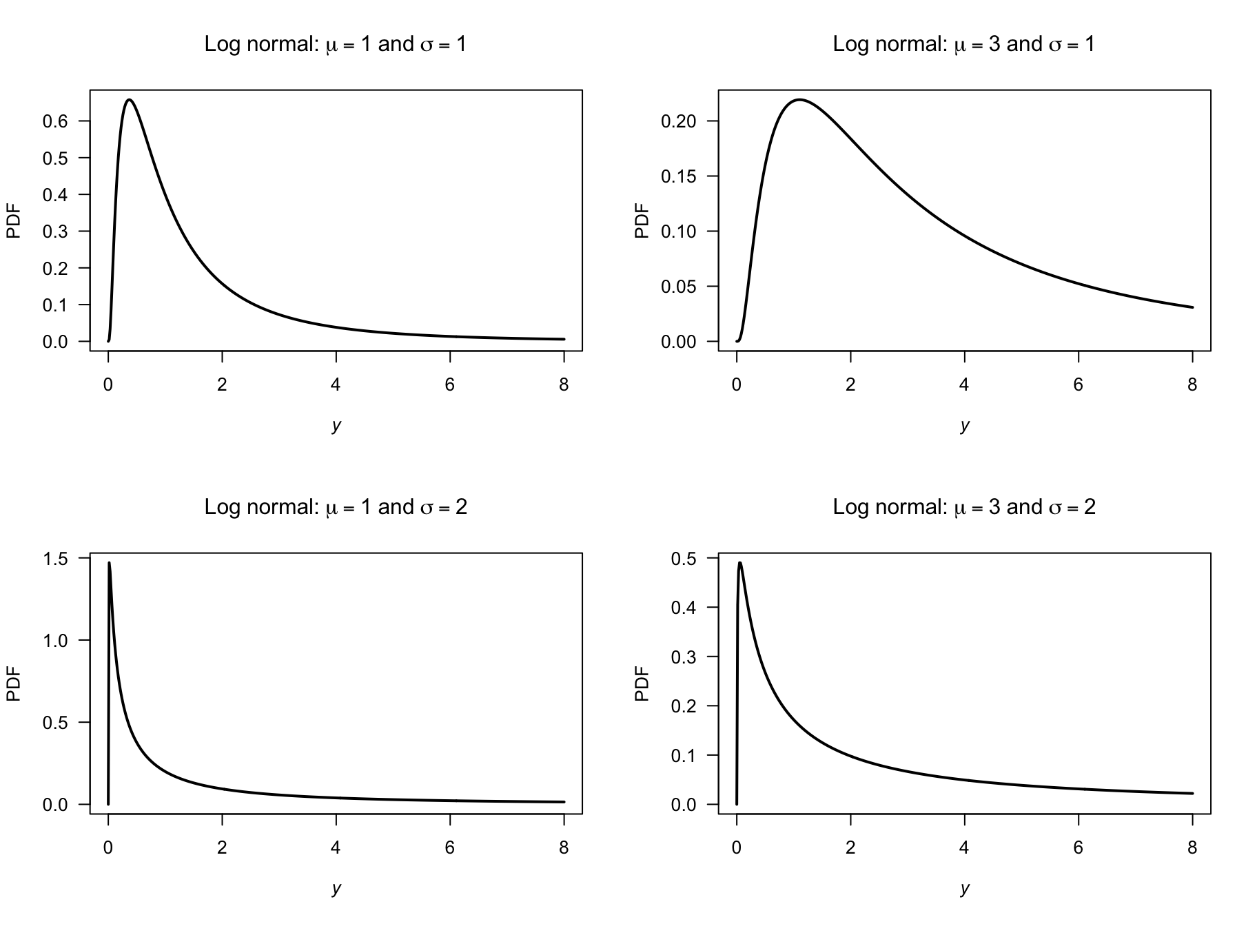

FIGURE F.69: Log-normal distributions

(1 - plnorm(2, meanlog=2, sdlog=2)) / 
  (1 - plnorm(1, meanlog=2, sdlog=2))
#> [1] 0.8834182

Exercise 9.16. See that $Y\in\{0, 1, \sqrt{2}, \sqrt{3}, 2\}$ and so \[ \Pr(Y = y) = \binom{4}{y^2} (0.2)^{y^2} (0.8)^{4 - y^2} \quad \text{for $y = 0, 1, \sqrt{2}, \sqrt{3}, 2$}. \]

Exercise 9.17.

First, see the relationships: \[\begin{align*} X = 1 &\to Y = (X - 3)^2 = 4;\\ X = 2 &\to Y = (X - 3)^2 = 1;\\ X = 3 &\to Y = (X - 3)^2 = 0;\\ X = 4 &\to Y = (X - 3)^2 = 1. \end{align*}\] So adding probabilities as appropriate: \[ p_Y(y) = \begin{cases} 9/30 & \text{for $y = 0$};\\ 20/30 & \text{for $y = 1$};\\ 1/30 & \text{for $y = 4$}. \end{cases} \]

Exercise 9.21. For the given beta distribution, $\operatorname{E}[V] = 0.287/(0.287 + 0.926) = 0.2366...$ and $\operatorname{var}[V] = 0.08161874$.

$\operatorname{E}[S] = \operatorname{E}[4.5 + 11V] = 4.5 + 11\operatorname{E}[V] = 7.10$ minutes. $\operatorname{var}[S] = 11^2\times\operatorname{var}[V] = 9.875$ minutes².
$V\in (4.5, 15.5)$. See Fig. F.70.
This corresponds to $V = 10.5/11 = 0.9545455$, so $\Pr(S > 15) = \Pr(V > 0.9545455) = 0.01745087$.
With $V$, the largest 20% correspond to $V = 0.004080076$, so that $S = 4.544881$; the quickest $20%$ are within $4.54\,\text{mins}$.

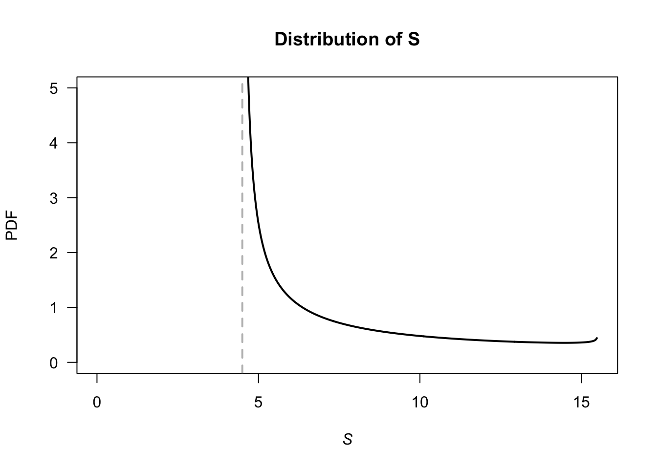
FIGURE F.70: Service times

#> [1] 0.01745087
#> [1] 4.50408

Exercise 9.6. Care is needed with the interval: it is not 1:1.

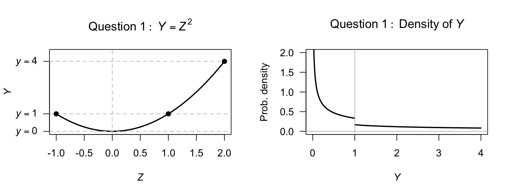
FIGURE F.71: Question 1.

Note that $Y$ is defined over $0 < Y < 4$, and the transformation is not a 1:1 transformation (Fig. 1, left panel) over these values. To use the distribution function method, see that $0 < y < 1$ corresponds to $-\sqrt{Y} < z < \sqrt{Y}$, but $1 \le y \le 4$ corresponds to $-1 < z <\sqrt{Y}$. For $y < 1$: \[ F_Y(y) = \Pr(Y \le y) = \Pr(-\sqrt{y} < z < \sqrt{y}\,) = \int_{-\sqrt{y}}^{\sqrt{y}} \frac{1}{3}\, dz = \frac{2\sqrt{y}}{3}\quad \text{for $0 < y < 1$}. \] For $1 < y < 4$, start by writing $F_Y(y) = \Pr(Y \le y)$, but then take care to include $\Pr(Y < 1)$! \[ F_Y(y) = \Pr(Y \le 1) + \Pr(1 < Y < y) = \frac{2}{3} + \Pr(1 < z < \sqrt{y}\,) = \frac{2}{3} + \int_{1}^{\sqrt{y}} \frac{1}{3}\, dz = \frac{1 + \sqrt{y}}{3}. \] Hence (noting carefully where $y = 1$ in the PDF): \[ F_Y(y) = \begin{cases} 0 & \text{for $y \le 0$};\\ \frac{2\sqrt{y}}{3} & \text{for $0 \le y < 1$};\\ \frac{1 + \sqrt{y}}{3} & \text{for $1 \le y < 4$};\\ 1 & \text{for $y \ge 4$} \end{cases} \quad\text{so differentiating:}\quad f_Y(y) = \begin{cases} \frac{1}{3\sqrt{y}} & \text{for $0 < y < 1$};\\ \frac{1}{6\sqrt{y}} & \text{for $1 \le y < 4$}. \end{cases} \]
For all values of $Y$, the PDF is non-negative. In addition, $\int_Y f_Y(y)\, dy = 1$.
See Fig. F.71 (right panel).

Exercise 9.24. We have \[ f_X(x) = \begin{cases} 2x/3 & \text{for $0 \le x \le 1$}\\ (3 - x)/3 & \text{for $1 < x \le 3$} \end{cases} \] and hence \[ F_X(x) = \begin{cases} 0 & \text{for $x < 0$}\\ x^2/3 & \text{for $0 \le x \le 1$}\\ (6x - x^2 - 3)/6 & \text{for $1 < x \le 3$}\\ 1 & \text{for $x > 3$.} \end{cases} \] Since $Y = 6 - 2x$, $\mathcal{R}_X = (0, 3)$ maps to $\mathcal{R}_Y = (0, 6)$; more specifically, $0 \le x \le 1$ maps to $4 \le y \le 6$ and $1 < x \le 3$ maps to $0 < y \le 4$. Then: \[\begin{align*} F_Y(y) &= \Pr(Y \le y)\\ &= \Pr\left( x \ge \frac{6 - y}{2}\right)\\ &= 1 - F_X\left( x \le \frac{6 - y}{2}\right). \end{align*}\] So, when $0 \le x \le 1$ (i.e., $4\le y \le 6$): \[ F_Y(y) = \frac{12y - y^2 - 24}{12} \] and when $1 < x \le 3$ (i.e., $0 < y \le 4$), $F_Y(y) = y^2/24$ so that (CHECK LESS THAN, LESS THAN OR EQUAL signs!!!!!!!!!!!) \[ f_Y(y) = \begin{cases} y/12 & \text{for $0 < y \le 4$}\\ (6 - y)/6 & \text{for $4 \le y \le 6$.} \end{cases} \]

Exercise 9.25. Not a 1:1 function so care is needed. $f_X(x)$ and $F_X(x)$ are given above. Since $Z = (X - 2)^2$, $\mathcal{R}_X = (0, 3)$ maps to $\mathcal{R}_Z = (0, 4)$; more specifically, $0 \le x \le 1$ maps to $1 \le z \le 4$ and $1 < x \le 3$ maps to $0 < z \le 1$. First consider the case $0\le z\le 1$: \[\begin{align*} F_Z(z) &= \Pr(Z \le y)\\ &= \Pr(2 - \sqrt{Z} \le X \le 2 + \sqrt{Z})\\ &= F_X(2 + \sqrt{z}) - F_X(2 - \sqrt{z})\\ &= 2\sqrt{z} / 3. \end{align*}\] Then, when $1\le z \le 4$: \[\begin{align*} F_Z(z) &= \Pr(Z \le z)\\ &= F_Z(1) + \Pr(2 - \sqrt{Z} \le X\le 1)\\ &= \frac{2}{3} + \frac{4\sqrt{z} - z - 3}{3}\\ &= \frac{4\sqrt{z} - z - 1}{3}. \end{align*}\] So we write \[ F_Z(z) = \begin{cases} 0 & \text{for $z < 0$}\\ 2\sqrt{z}/3 & \text{for $0 < z < 1$}\\ (4\sqrt{z} - z - 1)/3 & \text{for $1 < z < 4$}\\ 1 & \text{for $z > 4$.} \end{cases} \] Note that $F_Z(4) = 1$ and $F_Z(0) = 0$ as required. Furthermore, the two parts both give $F_Z(1) = 2/3$. Then, so that (CHECK LESS THAN, LESS THAN OR EQUAL signs!!!!!!!!!!!) \[ f_Z(z) = \begin{cases} 1/(3\sqrt{z}\,) & \text{for $0 < z \le 1$}\\ \left(2/\sqrt{z} - 1\right)/3 & \text{for $1 \le z \le 4$}. \end{cases} \]

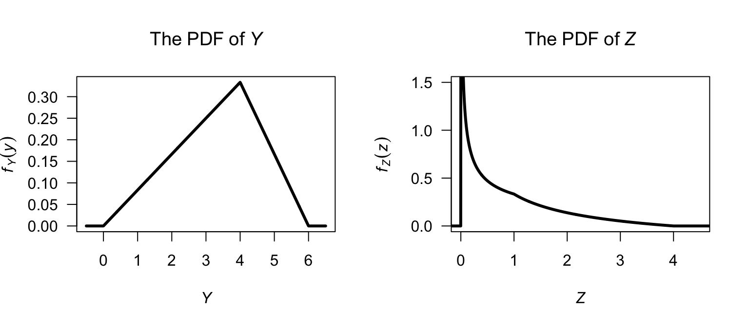
$The pdf of the transformed rvs\ $Y$ and\ $Z$.$

FIGURE F.72: The pdf of the transformed rvs $Y$ and $Z$.

Exercise 9.13. $f_V(v) = f_T(D/v)\, {\left|\frac{dT}{dV}\right|} = f_T(D/v) D/v^2$; and so \[ f_V(v) = \begin{cases} \displaystyle\frac{D(va + v\mu - D)}{a^2\,v^3} & \text{for $D/(\mu + \Delta) < v < D/\mu$}\\[6pt] \displaystyle\frac{D(va - v\mu + D)}{a^2\,v^3} & \text{for $D/\mu < v < D/(\mu - a)$} \end{cases} \] as in Fig. F.73 (left panel).

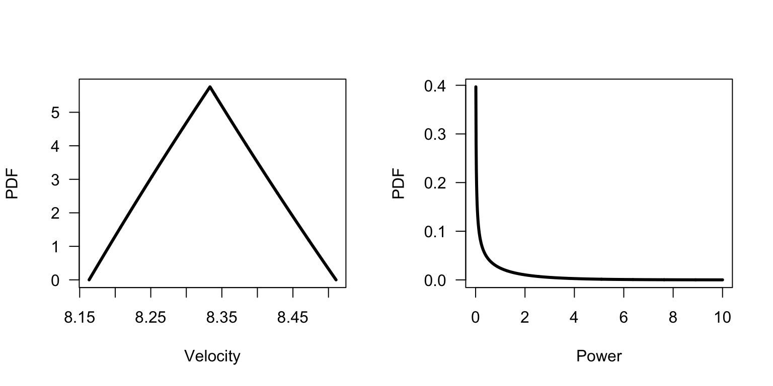
$The probability density function for the random variable\ $V$, the run velocity.$

FIGURE F.73: The probability density function for the random variable $V$, the run velocity.

Exercise 9.14. $f_P(p) = f_V(\sqrt{pR}) \frac{1}{2} \sqrt{R/p}$ and so \[ f_P(p) = \frac{\sqrt{R}}{\sqrt{2p\pi\sigma^2}} \exp\left\{-\frac{pR}{2\sigma^2}\right\} \] as shown in Fig. F.73 (right panel).

Exercise 9.26.

Taking logarithms of the product: \[ \log P = \log\!\left(\prod_{i=1}^n X_i\right) = \sum_{i=1}^n \log X_i. \]
Since $\log X_i \sim N(\mu_i, \sigma_i^2)$ independently, and the sum of independent normal random variables is normal (with means and variances adding), we have: \[ \log P = \sum_{i=1}^n \log X_i \sim N\!\left(\sum_{i=1}^n \mu_i,\; \sum_{i=1}^n \sigma_i^2\right). \] Since $P = \exp(\log P)$, and its logarithm is normally distributed, by definition: \[ P \sim \text{Log-normal}\!\left(\sum_{i=1}^n \mu_i,\; \sum_{i=1}^n \sigma_i^2\right). \]
From Part 2, with $\mu_i = 0.2$ and $\sigma_i^2 = 0.09$ for each $i = 1, \ldots, 10$: \[ \log P \sim N(10 \times 0.2,\; 10 \times 0.09) = N(2,\; 0.9) \] so $P \sim \text{Log-normal}(2, 0.9)$. Then: \[ \Pr(P > \exp 3) = \Pr(\log P > 3) = \Pr\!\left(Z > \frac{3 - 2}{\sqrt{0.9}}\right) = \Pr(Z > 1.054) \approx 0.146. \] Using R:

plnorm(exp(3), meanlog = 2, sdlog = sqrt(0.9), lower.tail = FALSE)
#> [1] 0.1459203

Exercise 9.27.

$F_X(x) = (x + 1)^2 /4$ for $-1 < x < 1$.
$F_Y(y) = y$ for $0 < y < 1$.
$f_Y(y) = 1$ for $0 < y < 1$.
Plots not shown. 1 . The $Y = |X|$ transformation effectively folds the left half of the distribution ($-1 < x < 0)$ onto the right half ($-1 < x < 0)$.

Exercise 9.29.

Since $A = pi R^2$, the inverse transform is $R = \sqrt{A/\pi}$ and $|dR/dA| = 1/(2\sqrt{\pi A}$. So \[ f_A(a) = \frac{\lambda \exp(-\lambda)\sqrt{a/\pi}}{2\sqrt{\pi\,a}} \quad\text{for $a > 0$.} \]
Since $A = \pi R^2$, $A = 200$ corresponds to $R = \sqrt{200/\pi})$: 1 - pexp(sqrt(200/pi), rate = 0.2), or about $0.203$.

lambda <- 0.2

fA <- function(a)
{
    lambda * exp(-lambda * sqrt(a/pi)) / (2 * sqrt(pi * a))
}

curve(fA, las = 1, ylim = c(0, 0.01),
      from = 0.1, to = 1000,
      xlab = expression(Area~(m^2)),
      ylab = "Probability density",
      main = "PDF of oil-spill area")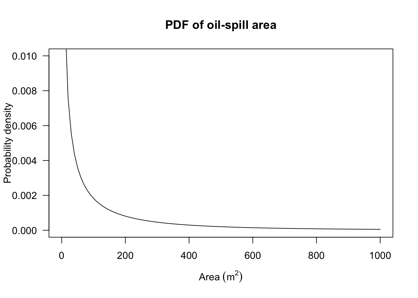

Exercise 9.28.

$T_a = 2531.7/V_A$ and $|d T_A/d V_A| = 2531.7/V_A^2$; so \[ f_V(v) = \frac{2531.7}{36\sqrt{2\pi}\, v^2} \exp\left(-\frac{(\frac{2531.7}{v} - 2500)^2}{2\times 26^2}\right) \] for $v > 0$.
Similar to 2.
Not normally distributed, but looks similar.

# Part 4
num_sims <- 10000

TA <- rnorm(num_sims, mean = 250, sd = 36)
TB <- rnorm(num_sims, mean = 280, sd = 36)

VA <- 60 * 42.195 / TA
VB <- 60 * 42.195 / TB

V_difference <- VA - VB

hist(V_difference, las = 1,
     probability = TRUE,
     main = "Estimated PDF of V_A - V_B",
     xlab = "Speed difference (km/h)")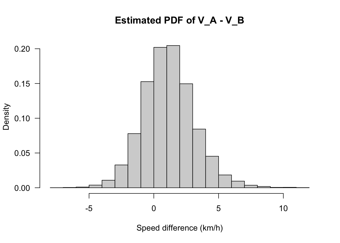

Exercise 9.30.

$R = \sqrt{A/\pi}$ so $dR/dA = 1/(2\sqrt{\pi A})$. Then: \[ f_A(a) = \begin{cases} (\sqrt{a/\pi} - 11) / (4\sqrt{\pi a}) & \text{for $121\pi \le a \le 144\pi$};\\ (13 - \sqrt{a/\pi}) / (4\sqrt{\pi a}) & \text{for $144\pi \le a \le 169\pi$}. \end{cases} \] for $a > 0$. Not triangular, but looks similar.

fA <- function(a){
    ans <- numeric(length(a))

    i1 <- (a >= 121*pi) & (a <= 144*pi)
    ans[i1] <- (sqrt(a[i1]/pi) - 11) /
        (4 * sqrt(pi * a[i1]))

    i2 <- (a > 144*pi) & (a <= 169*pi)
    ans[i2] <- (13 - sqrt(a[i2]/pi)) /
        (4 * sqrt(pi * a[i2]))
    ans
}

curve(fA, las = 1,
      from = 121*pi, to = 169*pi,
      xlab = expression(Area~("in"^2)),
      ylab = "Probability density",
      main = "PDF of pizza area")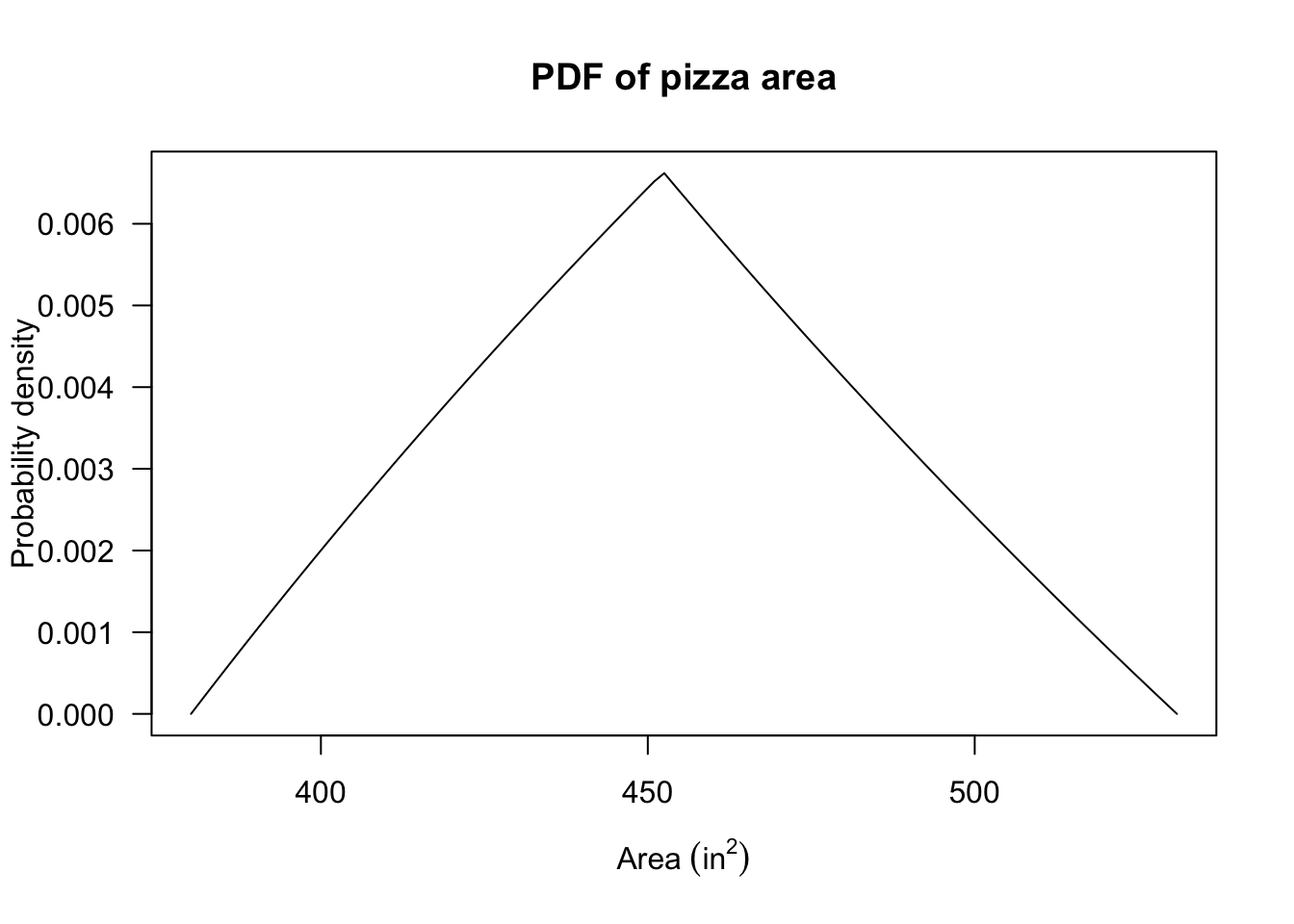

Exercise 9.31.

Write $U = \sqrt{2gh}$ ad $|dU/dH| = g/\sqrt{2gh}$; $f_H(h) = f_U(\sqrt{2gh}) g/\sqrt{2gh}$ in general.

If $U\sim N(15, 2^2)$, then \[ f_H(h) = \frac{g}{4\sqrt{\pi\, gh}}\exp\left(-\frac{(\sqrt{2gh} - 15)^2}{8}\right) \] for $h > 0$.
If $U\sim\Gamma(10, 1.5)$, then \[ f_H(h) = \frac{(\sqrt{2gh})^9\, \exp(-\sqrt{2gh}/1.5)}{\Gamma(10)\,1.5^{10}}\, \frac{g}{\sqrt{2gh}} \]
Plot below.
$\operatorname{E}[U^2] = \operatorname{var}[U] + (\operatorname{E}[U])^2$, so $\operatorname{E}[H] = (\operatorname{var}[U] + (\operatorname{E}[U])^2)/(2g)$. For the normal, $\operatorname{E}[H] = 11.68\,\text{m}$. For the gamma, $\operatorname{E}[H] = 12.63\,\text{m}$.

g <- 9.8

fH_norm <- function(h){
    u <- sqrt(2 * g * h)
    dnorm(u, mean = 15, sd = 2) * g / u
}

fH_gamma <- function(h){
    u <- sqrt(2 * g * h)
    dgamma(u, shape = 10, scale = 1.5) * g / u
}

curve(fH_norm, las = 1,
      from = 0, to = 30,
      ylim = c(0, 0.2),
      xlab = "Maximum height (m)",
      ylab = "Probability density",
      lwd = 2)

curve(fH_gamma,
      add = TRUE,
      lwd = 2,
      lty = 2)

legend("topright",
       legend = c("Normal velocity", "Gamma velocity"),
       lwd = 2,
       lty = c(1, 2),
       bty = "n")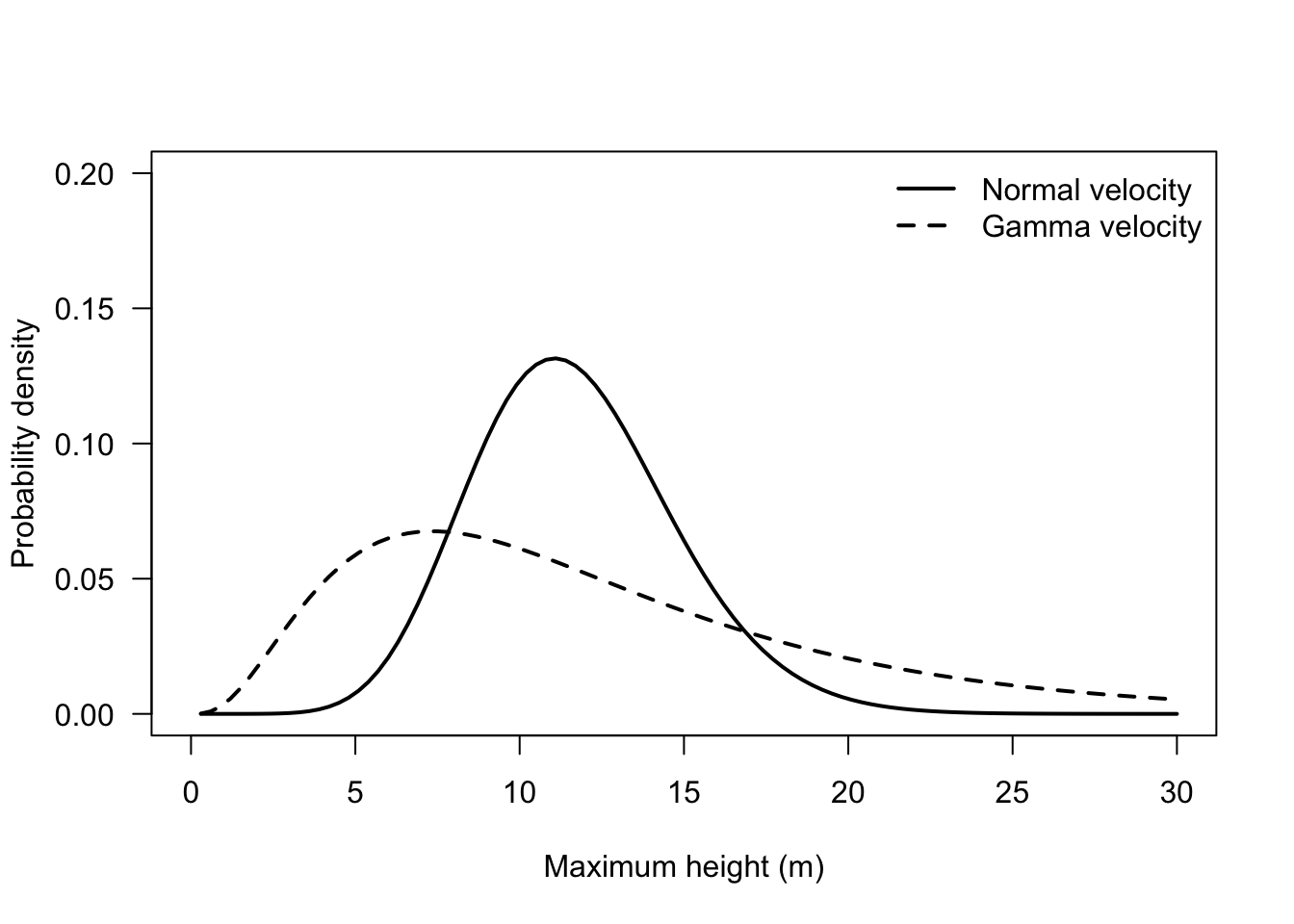

F.9 Answers for Chap. 10

Exercise 10.1.

This corresponds to the cell $X = 1, Y = 2$: $5/24\approx 0.208333$.
$\Pr(X + Y \le 1) = \Pr(X = 0, Y = 0) + \Pr(X = 0, Y = 1) + \Pr(X = 1, Y = 0) = 1/2$.
$\Pr(X > Y) = \Pr(X = 1, Y = 0) = 1/4$.
Write: \[ p_X(x) = \begin{cases} 7/24 & \text{if $x = 0$};\\ 17/24 & \text{if $x = 1$}. \end{cases} \]
Only consider the column corresponding to $X = 1$: \[ p_{Y\mid X = 1}(y\mid x = 1) = \begin{cases} (1/4)/(17/24) = 6/17 & \text{if $y = 0$};\\ (1/4)/(17/24) = 6/17 & \text{if $y = 1$};\\ (5/24)/(17/24) = 5/17 & \text{if $y = 2$}. \end{cases} \]

Exercise 10.2.

$0$.
$9/15$.
When $Y = \{0, 1, 2, 3, 4\}$ then $X = \left\{\{1, 2, 3\}, \{1, 2, 3\}, \{2, 3\}, \{2, 3\}, \{3\}\right\}$; then: $(1 + 6 + 3 + 2 + 0)/15 = 12/15$.
$\Pr(Y = 0) = 1/15$; $\Pr(Y = 1) = 6/15$; $\Pr(Y = 2) = 4/15$; $\Pr(Y = 3) = 3/15$; $\Pr(Y = 4) = 1/15$.
$\Pr(X = 1) = 4/15$; $\Pr(X = 2) = 5/15$; $\Pr(X = 3) = 6/15$.
$\Pr(Y = 1\mid X = 1) = 2/4$; $\Pr(Y = 2\mid X = 1) = 1/4$; $\Pr(Y = 3\mid X = 1) = 1/4$.

Exercise 10.3.

$\int_0^2\!\!\!\int_0^1 x + y^2\, dy\, dx = 11/3$, so $k = 3/11$.
$\dfrac{3}{11} \int_1^2\!\!\!\int_{1/2}^1 x + y^2\, dy\, dx = 37/88\approx 0.42045$.
???
$\dfrac{3}{11} \int_0^2 x + y^2\, dy = 2(3x + 4)/11$ for $0 < x < 1$.
$\dfrac{3}{11} \int_0^1 x + y^2\, dx = 3(2y^2 + 1)/22$ for $0 < y < 2$.
$2(x + y^2) / [2(3x + 4)]$ for $0 < x < 1$, $0 < y < 2$.
$3(1 + y^2) / 14$ for $0 < y < 2$.
$2(x + y^2) / (2y^2 + 1)$ for $0 < x < 1$, $0 < y < 2$.
$2(x + 1)/3$ for $0 < x < 1$.
No.

Exercise 10.4.

$k = 1/7$.
$3/7\approx 0.42857$.
Same as above: $3/7$.
$2(x + 2)/7$ for $1 < x < 2$.
$(7 - 2y)/14$ for $-1 < y < 1$ for $1 < x < 2$, $-1 < y < 1$.
$(2 + x - y)/[(2(x + 2)]$ for $1 < x < 2$, $-1 < y < 1$.
$(3 - y)/6$ for $-1 < y < 1$.
$2(2 + x -y)/(7 - 2y)$ for $1 < x < 2$.
$2(1 + x)/5$ for $1 < x < 2$.
No.

Exercise 10.5.

Exercise 10.6. 1. Write as: \[\begin{align*} f_{X, Y}(-1, y) &= f_{Y\mid X = -1}(y)\cdot p_X(X = -1) = \frac{1}{2}\times\frac{3}{10} = \frac{3}{20}\quad\text{for $-1 < y < 1$};\\ f_{X, Y}(1, y) &= f_{Y\mid X = -1}(y)\cdot p_X(X = 1) = \frac{1}{4} \times\frac{7}{10} = \frac{7}{40}\quad\text{for $-2 < y < 2$}. \end{align*}\] 2. $\Pr(Y > 1) = \Pr(Y > 1\mid X = -1) + \Pr(Y > 1 \mid X = -2)$ by the Law of Total Probability. Hence: $\left(\frac{3}{20}\times 0\right) + \left(\frac{7}{40}\times\frac{1}{4}\right) = \frac{7}{160} = 0.04375$, since the conditional distributions are uniform distributions.

Exercise 10.7.

Exercise 10.8.

Need integral to be one: $\int_0^1\!\!\!\int_0^1 kxy\, dx\, dy = 1$, so $k = 4$.
Here: \[ 4 \int_0^{3/8}\!\!\!\int_0^{5/8} kxy\, dx\, dy = 225/4096\approx 0.05493. \]

Exercise 10.9.

$F_{Y\mid X = x}(y) = \int_0^y \frac{2(x + s)}{2x + 1}\, ds = \frac{2yx + y^2}{2x+1}$ for $0 < x < 1$ and $0 < y < 1$.
$F_{Y = 3/4\mid X = 1/3}(y) = 51/80$.
$f_{X,Y}(x, y) = f_{Y\mid X=x}(y) \cdot g_X(x) = x + y$, for $0 < x < 1$, $0 < y < 1$.
$\Pr(Y < X) = \int_0^1\int_y^1 x + y\,dx\, dy = 1/2.$.

Exercise 10.10.

Construct table (below) from listing all four outcomes.
We get \[ p_X(x) = \begin{cases} 1/4 & \text{for $x = 0$};\\ 1/2 & \text{for $x = 1$};\\ 1/4 & \text{for $x = 2$}. \end{cases} \]
When given $Y = 1$, then the probability function is non-zero for $x = 1, 2$: \[ p_{X\mid Y = 1}(x \mid Y = 1) = \begin{cases} 1/2 & \text{for $x = 1$};\\ 1/2 & \text{for $x = 2$}; \end{cases} \]
Not independent; for instance, when $Y = 0$, $\Pr(X) > 0$ for $x = 0, 1$, in constrast to when $Y = 1$.

. $X = 0$ $X = 1$ $X = 2$

$Y = 0$ $1/4$ $1/4$ $0$

$Y = 1$ $0$ $1/4$ $1/4$

.	\(X = 0\)	\(X = 1\)	\(X = 2\)
\(Y = 0\)	\(1/4\)	\(1/4\)	\(0\)
\(Y = 1\)	\(0\)	\(1/4\)	\(1/4\)

Exercise 10.11. The joint probability function for $C$ and $D$ is shown in Table F.3. For example:

A minimum of 2 and a maximum of 1 is impossible; this makes no sense (hence probability is zero).
A minimum of 3 and a maximum of 4 can happen in two ways: a 4 on the first die and a 3 on the other, or a 3 on the first die and a 4 on the other.
A minimum and a maximum of 2 can only happen one way: both dice show a 2.

The joint distribution for $C$ and $D$ is therefore:

	$C = 0$	$C = 1$
$D = 0$	$6/36$	$6/36$
$D = 1$	$12/36$	$12/36$

Then, the marginal distribution for $B$ (the minimum) is \[ f_B(b) = \begin{cases} 11/36 & \text{for $b = 1$};\\ 9/36 & \text{for $b = 2$};\\ 7/36 & \text{for $b = 3$};\\ 5/36 & \text{for $b = 4$};\\ 3/36 & \text{for $b = 5$};\\ 1/36 & \text{for $b = 6$} \end{cases} \] which is easily confirmed as a valid PMF.

TABLE F.3: The minimum and maximum from two rolls of a die
	$\text{min} = 1$	$\text{min} = 2$	$\text{min} = 3$	$\text{min} = 4$	$\text{min} = 5$	$\text{min} = 6$
$\text{max} = 1$	1/36	0/36	0/36	0/36	0/36	0/36
$\text{max} = 2$	2/36	1/36	0/36	0/36	0/36	0/36
$\text{max} = 3$	2/36	2/36	1/36	0/36	0/36	0/36
$\text{max} = 4$	2/36	2/36	2/36	1/36	0/36	0/36
$\text{max} = 5$	2/36	2/36	2/36	2/36	1/36	0/36
$\text{max} = 6$	2/36	2/36	2/36	2/36	2/36	1/36

Exercise 10.12.

See Fig. F.74.
Integrate correctly! $\int_0^2 \!\!\!\int_0^{2 - x} x(y + 1)\,dy \, dx = 2$, so $c = 1/2$.
$\Pr(Y < 1 \mid X > 1) = \Pr(Y < 1 \cap X > 1)/\Pr(X > 1)$. First, $f_X(x) = (1/2) \int_0^{2 - x} x(y + 1)\,dy = (1/4)(x^3 - 6x^2 + 8x)$ for $0 < x < 2$. So $\Pr(X > 1) = 7/16 = 0.4375$. Also, \[ \Pr(Y < 1 \cap X > 1) = (1/2) \int_1^2 \!\!\!\int_0^{2 - x} x(y + 1)\,dy \, dx = 7/16. \] Then, $\Pr(Y < 1 \mid X > 1) = 1$, which makes sense from the diagram (if $X > 1$, $Y$ must be less than 1).
$\Pr(Y < 1 \mid X > 0.25) = \Pr(Y < 1 \cap X > 0.25)/\Pr(X > 0.25)$. Using results from above, $\Pr(X > 0.25) = 3871/4096 = 0.945068$ and $\Pr(Y < 1 \cap X > 0.25) = 0.945$. So $\Pr(Y < 1 \mid X > 0.25) = \Pr(Y < 1 \cap X > 0.25)/\Pr(X > 0.25)$.
First, $f_Y(y) = \frac{1}{2} \int_0^{2 - y} x(y + 1)\, dx = \frac{1}{4}(y + 1)(y - 2)^2$. Then, \[ \Pr(Y < 1) = \int_0^1 \frac{1}{4}(y + 1)(y - 2)^2\, dy = \frac{13}{16}\approx 0.8125. \]

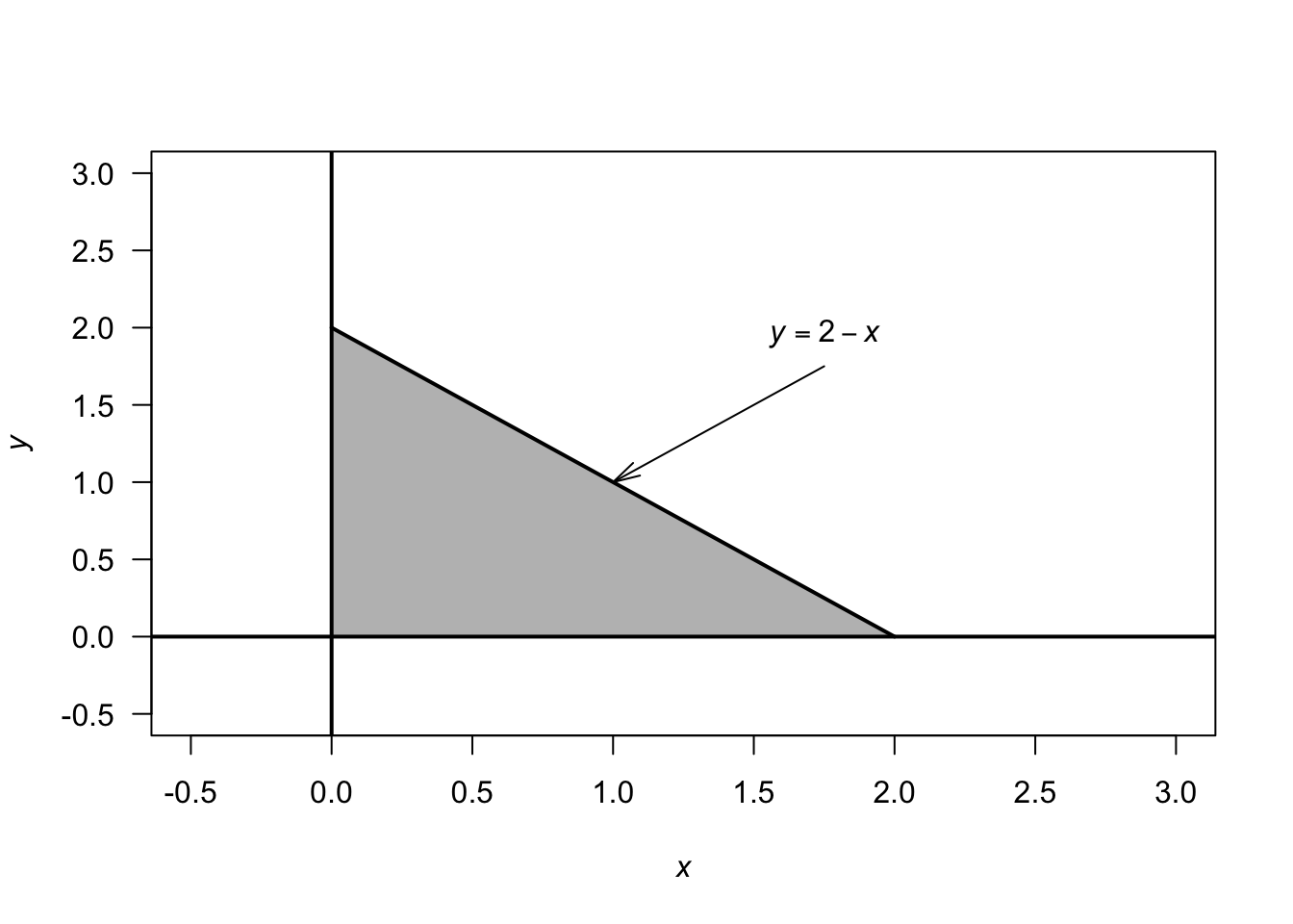
FIGURE F.74: The region where $X$ and $Y$ have positive probability

Exercise 10.13.

Proceed: \[\begin{align*} 1 &= k\int_0^1\!\!\!\int_0^{\sqrt{y}} (1 - x)y\, dx\, dy\\ &= k\int_0^1\!\!\!\int_{x^2}^{1} (1 - x)y\, dy\, dx\\ &= \frac{k}{2}\int_0^1 (1 - x) (1 - x^4) \, dx = \frac{7k}{30}, \end{align*}\] so that $k = 30/7\approx 4.285714$.
Being careful with the integration limits again (draw a diagram!): \[\begin{align*} \Pr(X > Y) &= \int_0^1 \!\int_y^{\sqrt{y}} f_{X, Y}(x, y)\, dx\, dy\\ &= \int_0^1 \!\int_x^{x^2} f_{X, Y}(x, y)\, dy\, dx\\ &= \frac{15}{7} \int_0^1 (x - 1) x^2 (x^2 - 1)\, dx = 3/28\approx 0.1071429. \end{align*}\]
First find the marginal distribution of $X$: \[ f_X(x) = \int_{x^2}^1 f_{X, Y}(x, y)\, dy = \frac{15}{7} (x - 1)(x^4 - 1), \] and so \[ \Pr(X > 0.5) = \frac{15}{7} \int_{1/2}^1 (x - 1)(x^4 - 1)\, dx = \frac{183}{896}\approx 0.2042411. \]

Exercise 10.14.

$1 = k\int_0^1 \int_0^{1 - x} y(2 + 2y)\, dy\, dx = 5/24$, so that $k = 24/5 = 4.8$.
More complicated region. Either: $\Pr(X > Y) = \frac{24}{5} \int_0^{1/2}\int_0^x y(x + 2y) \, dy \, dx + \frac{24}{5} \int_{1/2}^1\int_0^{1-x} y(x + 2y) \, dy \, dx$. Or: $\Pr(X > Y) = \frac{24}{5} \int_0^{1/2}\int_{y}^{1 - y} y(x + 2y) \, dy \, dx$. Either way: $1/5$.
$f_X(x) = \int_0^{1 - x} y(x + 2y)\, dy = \frac{4}{5}(4 - x)(x - 1)^2$ for $0 < x < 1$. So $\Pr(X > 0.5) = \int_0^{0.5} \frac{4}{5}(4 - x)(x - 1)^2\,dx = 9/80 = 0.1125$.

Exercise 10.16. 1. $f_X(x) = x(1 - x^2)/2$ for $0 < x < 1$. 2. $f_{X\mid Y=y}(x) = 2xy/(x(1-x^2))$ for $0<y<\sqrt{1 - x^2}$. 3. $f_{X\mid Y=1/2}(x) = 3y/2$ for $0 < y < \sqrt{3}/2$.

Exercise 10.17. 1. $f_Y(y) = 2 + 2y - 3y^2/2$ for $0 < y < 1$. $f_X(x) = 3x^2/2$ for $0<x<1$; $f_X(x) = x + (1/2)$ for $1 < x < 2$. 2. $f_{Y\mid X=x}(y) = 2(x + y)/(3x^2)$ for $0<y<x$ and $0<x<1$; $f_{Y\mid X=x}(y) = 2(x + y)/(2x + 1)$ for $0<y<1$ and $1<x<2$. 3. $f_{Y\mid X=1}(x) = 2(1 = Y0/3$ for $0 < y < 1$.

Exercise 10.24. See that $y_1 > 0$ and $y_2 > 0$. Since the random variable $X_1$ and $X_2$ are iid, the joint PDF of $X_1$ and $X_2$ is \[ f_{X_1, X_2}(x_1, x_2) = \exp(-x_1) \cdot \exp(-x_2) = \exp\left(-(x_1 + x_2)\right) \quad \text{for $x_1, x_2 > 0$}. \] Inverting the transformations gives \[ x_1 = \frac{y_1 y_2}{1 + y_2} \quad\text{and}\quad x_2 = \frac{y_1}{1 + y_2}. \] The Jacobian requires the four partial derivatives: \[ \begin{array}{ll} \displaystyle \frac{\partial x_1}{\partial y_1} = \frac{y_2}{1+y_2};\quad & \quad\displaystyle \frac{\partial x_1}{\partial y_2} = \frac{y_1(1+y_2) - y_1 y_2}{(1+y_2)^2} = \frac{y_1}{(1+y_2)^2};\\[12pt] \displaystyle \frac{\partial x_2}{\partial y_1} = \frac{1}{1+y_2};\quad & \quad\displaystyle \frac{\partial x_2}{\partial y_2} = \frac{-y_1}{(1+y_2)^2}. \end{array} \] So the Jacobian determinant is \[\begin{align*} \det J &= \left( \frac{y_2}{1+y_2} \cdot \frac{-y_1}{(1+y_2)^2} \right) - \left( \frac{1}{1+y_2} \cdot \frac{y_1}{(1+y_2)^2} \right)\\ &= \frac{-y_1 y_2 - y_1}{(1+y_2)^3}\\ &= \frac{-y_1(y_2 + 1)}{(1+y_2)^3}. \end{align*}\] Finally, substitute $x_1$ and $x_2$ and $\det J$ into the formula: \[ f_{Y_1, Y_2}(y_1, y_2) = \exp(-(x_1 + x_2)) \cdot \left| \frac{-y_1}{(1 + y_2)^2} \right|. \] Since $x_1 + x_2 = y_1$, write \[ f_{Y_1, Y_2}(y_1, y_2) = \frac{y_1 \exp(-y_1)}{(1+y_2)^2}\quad\text{for $y_1 > 0$ and $y_2 > 0$}. \]

Exercise 10.25. Consider the two one-to-one transformations (where $Y_2 = X_2$ is just a dummy transformation since we need to work with two transformations): \[\begin{align} y_1 &= x_1 + x_2 = u_1(x_1, x_2)\\ y_2 &= x_2\phantom{{} + x_2} = u_2(x_1, x_2) \end{align}\] which map the points in $\mathcal{R}^2_X$ onto \[ \mathcal{R}^2_Y = \left\{ (y_1, y_2)\mid y_1 = 0, 1, 2, \dots; y_2 = 0, 1, 2, \dots, y_1\right\}. \] $Y_2$ is a dummy transform, and is chosen to be very simple; any second transform could be chosen (since it is not of direct interest). The inverse functions are \[\begin{align*} x_1 &= y_1 - y_2 = w_1(y_1, y_2)\\ x_2 &= y_2 \phantom{{} - y_2} = w_2(y_2) \end{align*}\] by rearranging the original transformations. Then the joint probability function of $Y_1$ and $Y_2$ is \[\begin{align*} p_{Y_1, Y_2}(y_1, y_2) &= p_{X_1, X_2}\big( w_1(y_1, y_2), w_2(y_1, y_2)\big) \\ &= \frac{\lambda_1^{y_1 - y_2}\lambda_2^{y_2} \exp(-\lambda_1 - \lambda_2)}{(y_1 - y_2)! y_2!}\quad \text{for $(y_1, y_2)\in \mathcal{R}^2_Y$}. \end{align*}\] Recall that we seek the probability function of just $Y_1$, so we need to find the marginal probability function of $p_{Y_1, Y_2}(y_1, y_2)$. The marginal probability function of $Y_1$ is \[ p_{Y_1}(y_1) = \sum_{y_2 = 0}^{y_1} p_{Y_1, Y_2}(y_1, y_2) = \sum_{y_2 = 0}^{y_1} \frac{\lambda_1^{y_1 - y_2}\lambda_2^{y_2} \exp(-\lambda_1 - \lambda_2)}{(y_1 - y_2)!\, y_2!}. \] To simplify, first multiply and divide by $y_1!$: \[\begin{align*} p_{Y_1}(y_1) &= \frac{\exp(-\lambda_1 - \lambda_2)}{y_1!} \sum_{y_2 = 0}^{y_1} \frac{y_1!}{(y_1 - y_2)!\, y_2!} \lambda_1^{y_1 - y_2}\lambda_2^{y_2}\\ &= \frac{\exp(-(\lambda_1 + \lambda_2))}{y_1!} \sum_{y_2 = 0}^{y_1} \binom{y_1}{y_2} \lambda_1^{y_1 - y_2}\lambda_2^{y_2}.\\ \end{align*}\] Then, using the binomial theorem (Sect. B.1), this simplifies to \[\begin{align*} p_{Y_1}(y_1) &= \frac{\exp\big(-(\lambda_1 + \lambda_2)\big)}{y_1!} (\lambda_1 + \lambda_2)^{y_1} \\ &= \frac{\exp(-\Lambda)}{y_1!} \Lambda^{y_1} \quad\text{for $y_1 = 0, 1, 2, \dots$} \end{align*}\] where $\Lambda = \lambda_1 + \lambda_2$. This is the probability function of a Poisson random variable (Def. 6.12) with mean $\Lambda$. Thus $Y_1 = X_1 + X_2$ has a Poisson distribution with a mean of $\lambda_1 + \lambda_2$: the sum of two independent Poisson random variables is also a Poisson random variable.

Exercise 10.26. $f_{Y_2}(y_1) = 0.1$ for $y_1 = 0$, $f_{Y_2}(y_1) = 0.6$ for $y_1 = 1$, $f_{Y_2}(y_1) = 0.2$ for $y_1 = 2$, $f_{Y_2}(y_1) = 0.1$ for $y_1 = 3$.

Exercise 10.27. Three parts:

Case 1: $\int_{-y_1}^{y_1} (y_1^2 - y_2^2)/16)\, dy_2$ when $0<y_1<1$.
Case 2: $\int_{-y_1}^{2 - y_1} (y_1^2 - y_2^2)/16)\, dy_2$ when $1\le y_1<2$.
Case 3: $\int_{y_1 - 4}^{2 - y_1} (y_1^2 - y_2^2)/16)\, dy_2$ when $2\le y_1 < 3$.

Then \[ f_{y_1}(y_1) = \begin{cases} y_1^3/12 & \text{for $0 < y_1 < 1$} \\ y_1/4 - (1/6) & \text{for $1\le y_1 < 2$}\\ (-y_1^3 + 15y_1 - 18)/12 & \text{$2 \le y_1 < 3$.} \end{cases} \]

Exercise 10.28.

$\operatorname{E}[G] = 22\times 0.60 = 13.2$
$\operatorname{E}[B] = 22\times 0.4 = 8.8$.
$\Pr(T = 20)$: dpois(20, 22), or approx $0.08088$.
$\Pr(G = 14\mid T = 20)$: dbinom(14, 20, 0.60) or approx. $0.12441$.
$\operatorname{E}[S] = 6\operatorname{E}[G] + \operatorname{E}[B] = 88$.

num_sims <- 10000

T <- rpois(num_sims, 22)
G <- rbinom(num_sims, T, 0.60)
B <- T - G
S <- 6*G + B

# Parts 6 to 10
cat("Mean score:", mean(S), "\n")
#> Mean score: 88.0278
cat("Variance of score:", var(S), "\n")
#> Variance of score: 480.5197
cat("P(less than 100 points):", sum(S < 100)/num_sims, "\n")
#> P(less than 100 points): 0.7107
cat("P(exactly 87 points):", sum(S == 87)/num_sims, "\n")
#> P(exactly 87 points): 0.0187
hist(S, las = 1, freq = FALSE,
     xlab = "Points", main = "Histogram of points scored" )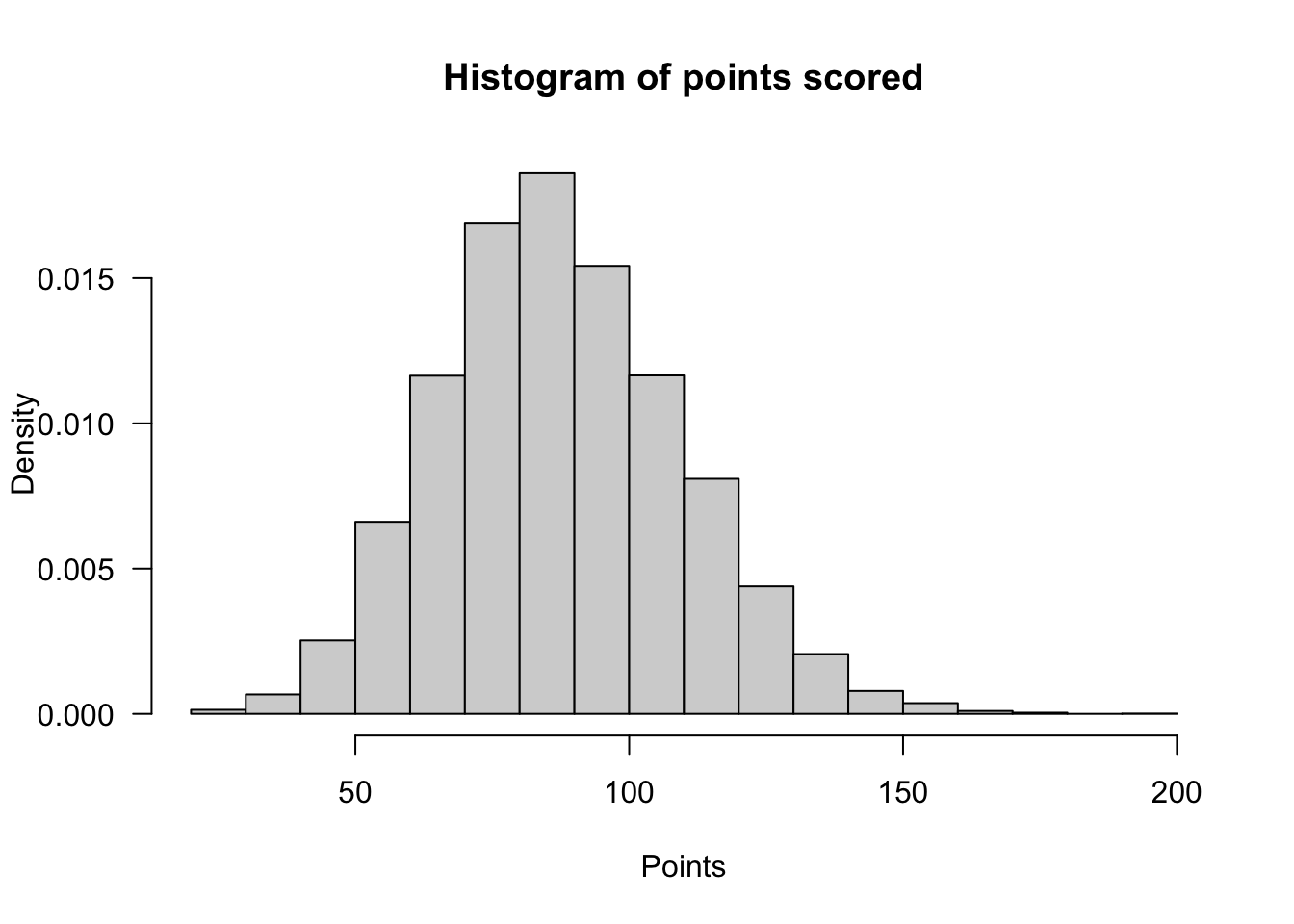

the mean final score;
the variance of the final score;
the probability that the team scores at least 100 points;
the probability that the team scores exactly 87 points;
the distribution of the team’s final score.

Exercise 10.29.

$\operatorname{E}[C\mid T] = 0.85T$, so \[ \operatorname{E}[C] = \operatorname{E}\big[\operatorname{E}[C\mid T]\big] = 0.85\operatorname{E}[T] = 0.85\times 4 = 3.4. \]
Since $T\sim\text{Poisson}(4)$, $\Pr(T = 3) = \exp(-4)\,4^3/3! = 0.19537$.
Given $T = 4$, then $C\mid T=4\sim\text{Binomial}(4, 0.85)$. Hence, $\Pr(C = 4\mid T = 4) = 0.85^4 = 0.52201$.
$\operatorname{E}[S] = 4\operatorname{E}[T] + 2\operatorname{E}[C] + 2\operatorname{E}[P] + \operatorname{E}[F] = (4\times 4) + (3.4\times 2) + (2\times 2) + (0.1\times 1) = 26.9$

num_sims <- 10000
T <- rpois(num_sims, 4)
C <- rbinom(num_sims, T, 0.85)
P <- rpois(num_sims, 2)
F <- rpois(num_sims, 0.1)

S <- 4*T + 2*C + 2*P + F

# Part 5--9
cat("Mean score:", round(mean(S, 3)), "\n")
#> Mean score: 26
cat("Variance of score:", round(var(S), 4), "\n")
#> Variance of score: 141.5761
cat("Prob scoring more than 30:", 
    sum(S > 30)/num_sims, "\n")
#> Prob scoring more than 30: 0.3462
cat("Prob of 20 points exactly:", 
    sum(S == 20)/num_sims, "\n")
#> Prob of 20 points exactly: 0.0634
hist(S, las = 1, freq = FALSE,
     xlab = "Points", main = "Histogram of points scored" )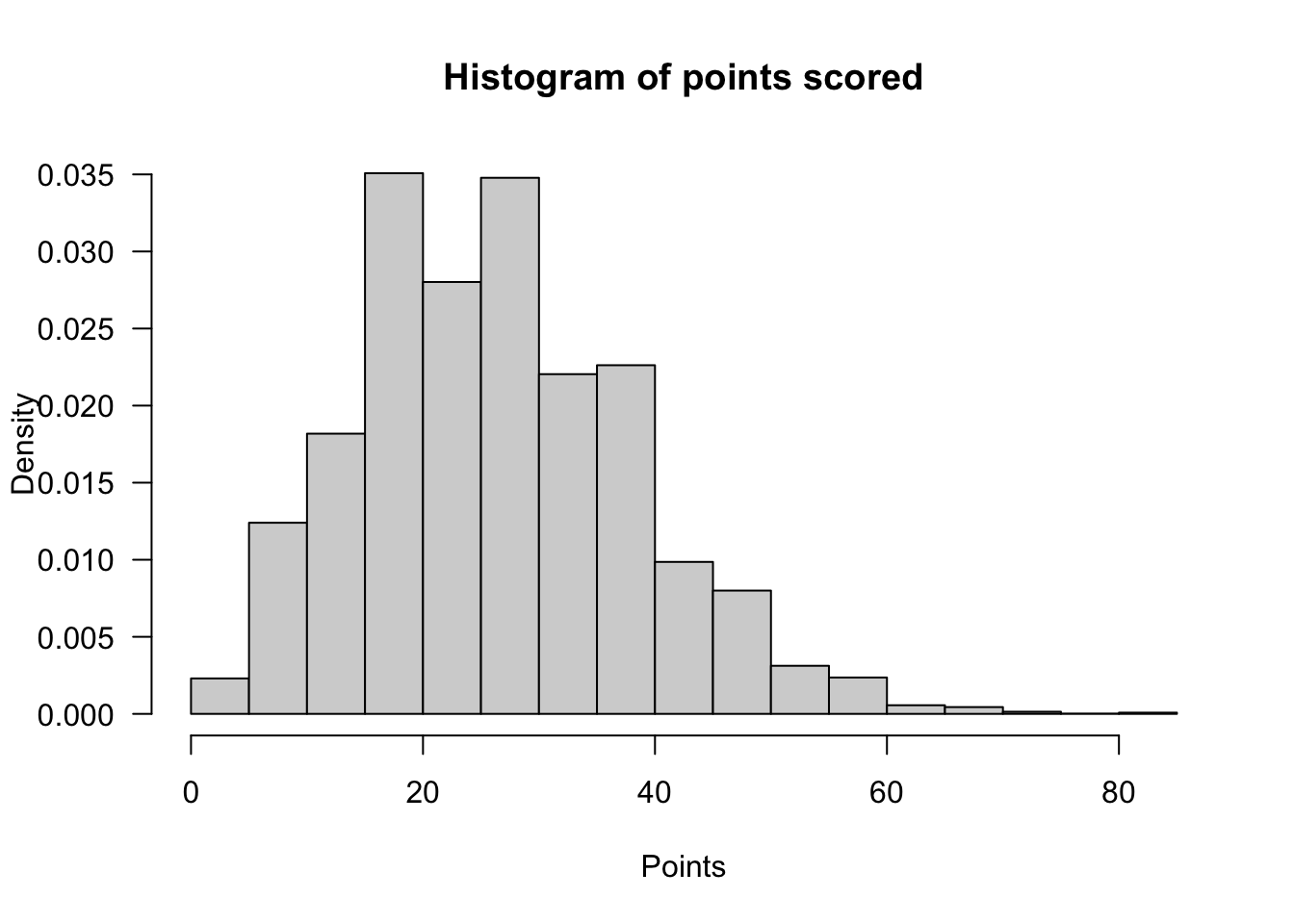

F.10 Answers for Chap. 11

Exercise 11.1.

The Jacobian: \[ J = \det \begin{bmatrix} \cos\theta & -r\sin\theta \\ \sin\theta & r\cos\theta \end{bmatrix} = r(\cos^2\theta + \sin^2\theta) = r. \] The joint PDF: \[ f_{R, \Theta}(r, \theta) = \left( \frac{1}{2\pi} e^{-\frac{1}{2}r^2} \right) \cdot r. \]

Exercise 11.2.

$\operatorname{E}[\overline{X}] = \operatorname{E}[(X_1 + X_2 + \cdots + X_n)/n] = [\operatorname{E}[X_1] + \operatorname{E}[X_2] + \cdots + \operatorname{E}[X_n])/n = (n \mu)/n = \mu$.
$\operatorname{var}[\overline{X}] = \operatorname{var}[(X_1 + X_2 + \cdots + X_n)/n] = (\operatorname{var}[X_1] + \operatorname{var}[X_2] + \cdots + \operatorname{var}[X_n])/n^2 = (n \sigma^2)/n^2 = \sigma^2/n$.

Exercise 11.3.

$\operatorname{E}[U] = \mu_x - \mu_Z$; $\operatorname{E}[V] = \mu_x - 2\mu_Y + \mu_Z$.
$\operatorname{var}[U] = \sigma^2_x + \sigma^2_Z$; $\operatorname{E}[V] = \sigma^2_x + 4\sigma^2_Y + \sigma^2_Z$.
Care is needed! \[\begin{align*} \text{Cov}[U, V] &= \operatorname{E}[UV] - \operatorname{E}[U]\operatorname{E}[V]\\ &= \operatorname{E}[X^2 - 2XY + XZ - XZ + 2YZ - Z^2] - \\ &\qquad (\mu_X^2 + 2\mu_X\mu_Y + \mu_X\mu_Z - \mu_X\mu_Z - 2\mu_Y\mu_Z - \mu^2_z)\\ &= (\operatorname{E}[X^2] - \mu_X^2) - 2(\operatorname{E}[XY] - \operatorname{E}[X]\operatorname{E}[Y]) + 2(\operatorname{E}[YZ] - \mu_Y\mu_Z) -\\ &\qquad (\operatorname{E}[Z^2] - \mu_Z^2) = \sigma^2_X - \sigma^2_Z, \end{align*}\] since the two middle terms become $-2\text{Cov}[X, Y] + 2\text{Cov}[Y, Z]$, are both are zero (as given).
The covariance is zero if $\sigma^2_X = \sigma^2_Z$.

Exercise 11.4.

First, $\Pr(X \mid Y = 2) = |x - 2|/11$. Then, the marginal distribution is \[ p(X\mid Y = 2) = \begin{cases} 2/3 & \text{for $x = 0$};\\ 1/3 & \text{for $x = 1$.} \end{cases} \] So $\operatorname{E}[X \mid Y = 2] = 1/3$.
First, $p_X(x) = \frac{1}{11}( |x - 1| + |x - 2| + |x - 3|)$ for $x = 0, 1, 2$; so $\Pr(X\ge 1) = 5/11$. The probability function is non-zero for $y = 1, 2, 3$. Then \[ p(Y\mid x\ge 1) = \begin{cases} 1/5 & \text{for $y = 1$};\\ 1/5 & \text{for $y = 2$};\\ 3/5 & \text{for $y = 3$}. \end{cases} \] Then, $\operatorname{E}[Y \mid X\ge 1] = 12/5$.

Exercise 11.5.

We find $f_X(x) = 1$ for $0 < x < 1$ and $f_Y(y) = 1$ for $0 < y < 1$.
We need some intermediate values: $\operatorname{E}[X] = \operatorname{E}[Y] = 1/2$; $\operatorname{var}[X] = \operatorname{var}[Y] = 1/12$; $\operatorname{E}[XY] = (9 - \alpha)/36$. Then $\text{Cov}[X, Y] = -\alpha/36$ and so $\text{Cor}[X, Y] = -\alpha/3$.
Independence if $f_X(x) \times f_Y(y) = f_{XY}(x, y)$, which occurs only when $\alpha = 0$.
$\Pr(X < Y) = \int_0^1\!\!\int_y^1 1 - \alpha(1 - 2x)(1 - 2y)\, dx\, dy = 1/2$.

Exercise 11.9. For an exponential distribution, the MGF is $M_X(t) = (1 - \beta t)^{-1}$. The MGF is a sum is the product of the MGFs (Theorem 5.9), so the MGF of $W = Z_1 + Z_2 + \cdots + Z_n$ is \[ M_W(t) = \prod_{i = 1}^n (1 - \beta t)^{-1} = (1 - \beta t)^{-n}, \] which is the MGF of a gamma distribution with parameters $n$ and $\beta$, as to be shown.

Exercise 11.11.

Adding: \[ p_X(x) = \begin{cases} 0.40 & \text{for $x = 0$};\\ 0.45 & \text{for $x = 1$};\\ 0.15 & \text{for $x = 3$}. \end{cases} \]
$\Pr(X \ne Y) = 1 - \Pr(X = Y) = 1 - (0.20) = 0.80$.
$X < Y$ only includes these five $(x, y)$ elements of the sample space: $\{ (0, 1), (0, 2), (0, 3); (1, 2), (1, 3)\}$. The sum of these probabilities is $0.65$. Given these five, only two sum to three ($(0, 3)$ and $(1, 2)$). So the probability of the intersection is $\Pr( \{0, 3\} ) + \Pr( \{1, 2\}) = 0.30$. The conditional probability is $0.30/0.65 = 0.4615385$; about $46$%.
No: For $X = 0$, the values of $Y$ with non-zero probability are $Y = 1, 2, 3$. However, for $X = 1$ (for example), the values of $Y$ with non-zero probability are $Y = 1, 2$.

Exercise 11.14.

$f(x_1, x_2, \dots, x_n) = 4^n \prod_{i = 1}^n x_i^3$.
$\Pr(X_1 < 1/2) = \int_0^{1/2} 4 x^3 \, dx = 1/16 = 0.0625$.
The prob. is $16^{-n}$.
Same as 3.

Exercise 11.16.

A table can be used to show the sample space (below). Looking for $X = 4$ we deduce that \[ p_Y(y|X = 4) = \begin{cases} 2/7 = 0.2857 & \text{for $y = 1$};\\ 2/7 & \text{for $y = 2$};\\ 2/7 & \text{for $y = 3$};\\ 1/7 & \text{for $y = 4$}. \end{cases} \] Hence we deduce that $\operatorname{E}[Y | X = 4] = 16/7\approx 2.2857$.

The table shows the values of $(x, y)$ (i.e, the entries are $(\text{max}, \text{min})$).

.	Die 1: 1	2	3	4	5	6
Die 2: 1	$(1, 1)$	$(2, 1)$	$(3, 1)$	$(4, 1)$	$(5, 1)$	$(6, 1)$
2	$(2, 1)$	$(2, 2)$	$(3, 2)$	$(4, 2)$	$(5, 2)$	$(6, 2)$
3	$(3, 1)$	$(3, 2)$	$(3, 3)$	$(4, 3)$	$(5, 3)$	$(6, 3)$
4	$(4, 1)$	$(4, 2)$	$(4, 3)$	$(4, 4)$	$(5, 4)$	$(6, 4)$
5	$(5, 1)$	$(5, 2)$	$(5, 3)$	$(5, 4)$	$(5, 5)$	$(6, 5)$
6	$(6, 1)$	$(6, 2)$	$(6, 3)$	$(6, 4)$	$(6, 5)$	$(6, 6)$


set.seed(108125)

numSims <- 10000; yCount <- 0
yVector <- array(dim = numSims)

for (i in 1:numSims){
  # Roll the dice
  Die1 <- sample(1:6, 1); Die2 <- sample(1:6, 1)
  
  x <- max( c(Die1, Die2) ); y <- min( c(Die1, Die2) )
  
  if (x == 4){
    yCount <- yCount + 1; yVector[yCount] <- y
  }
}

expY <- mean(yVector, na.rm = TRUE)
expY # Similar to what is expected
#> [1] 2.301363

Exercise 11.18.

annualRainfallList <- array( NA, dim = 1000)
for (i in 1:1000){
   rainAmounts <- array( 0, dim = 365) # Reset for each simulation

    wetDays <- rbinom(365, size = 1, prob = 0.32) # 1: Wet day
   locateWetDays <- which( wetDays == 1 )


   rainAmounts[locateWetDays] <- rgamma( n = length(locateWetDays),
                                         shape = 2,
                                         scale = 20)
   annualRainfallList[i] <- sum(rainAmounts)
}
# hist( annualRainfallList)

Days <- 1 : 365
prob <- (1 + cos( 2 * pi * Days/365) ) / 2.2

annualRainfallList2 <- array( NA, dim = 1000)
for (i in 1:1000){

  wetDays <- rbinom(365, size = 1, prob = prob) # 1: Wet day
  
  locateWetDays <- which( wetDays == 1 )
  
  rainAmounts2 <- array( 0, dim = 365)
  
  rainAmounts2[locateWetDays] <- rgamma( n = length(locateWetDays),
                                         shape = 2,
                                         scale = 20)
   annualRainfallList2[i] <- sum(rainAmounts2)
}
#hist( annualRainfallList2)

Days <- 1 : 365

probList <- array( dim = 365)
probList[1] <- 0.32

annualRainfallList3 <- array( NA, dim = 1000)

for (i in 1:1000){
  rainAmounts <- array( dim = 365 )

  for (day in 1:365) {
    if ( day == 1 ) {
      probList[1] <- 0.32
      wetDay <- rbinom(1, 
                       size = 1, 
                       prob = probList[1]) # 1: Wet day
      rainAmounts[1] <- rgamma( n = 1, shape = 2, scale = 20)

    } else {
      probList[i] <- ifelse( rainAmounts[day - 1] == 0,
                             0.15, 0.55)
      wetDay <- rbinom(1, 
                       size = 1, 
                       prob = probList[i]) # 1: Wet day

      if (wetDay) {
        rainAmounts[day] <- rgamma( n = 1,
                                    shape = 2,
                                    scale = 20)
      } else {
        rainAmounts[day] <- 0
      }
    }
  }
  annualRainfallList3[i] <- sum(rainAmounts)
}

Exercise 11.19.

$X + Y + Z = 500$: once the values of $X$ and $Y$ are known, the value of $Z$ is fixed (not variable).
See Fig. F.75 (left panel).
See Fig. F.75 (right panel).
Proceed: \[\begin{align*} 1 &= \int_{200}^{300} \!\! \int_{100}^{400 - y} k\,dx\,dy + \int_{100}^{200} \!\! \int_{300 - y}^{400 - y} k\,dx\,dy \\ &= 30\ 000, \end{align*}\] so that $k = 1/30\,000$.

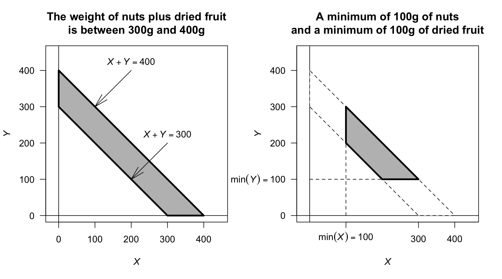
FIGURE F.75: The sample space for the mixture of nuts and dried fruit.

Answer for Exercise 11.20.

Let $W$, $A$, and $P$ denote the walnut, almond, and peanut weights (in grams). Since each packet contains $250\,\text{g}$, $W + A + P = 250$ implying $P = 250 - W - A$. Once $W$ and $A$ are specified, $P$ is determined.
We have $W \ge 0$, $A \ge 0$ and $0 \le P \le 100$. Then, since $P = 250 - W - A$, \[ 0 \le 250 - W - A \le 100 \quad \Rightarrow \quad 150 \le W + A \le 250. \] Hence the sample space is $\mathcal{R}_2 = \{(w,a) : w \ge 0, \; a \ge 0, \; 150 \le w + a \le 250\}$. This is a trapezoid in the $(W, A)$-plane with vertices $(150, 0), \quad (250, 0), \quad (0, 250), \quad (0, 150)$.
Adding the requirements $W \ge 25$ and $A \ge 25$ gives the feasible region as \[ \mathcal{R}_3 = \{(w,a) : w \ge 25, \; a \ge 25, \; 150 \le w + a \le 250\} \] with corners at $(125, 25), \quad (225, 25), \quad (25, 225), \quad (25, 125)$.
Assuming the weights are uniformly distributed over the feasible region with just the peanuts restriction, the area is \[ \text{Area}(\mathcal{R}_2) = \frac{1}{2}\cdot 250^2 - \frac{1}{2}\cdot 150^2 = 20\,000. \] So $f_{W, A}(w, a) = \frac{1}{20\,000}$ for $(w, a) \in \mathcal{R}_2$. Then, with additional lower bounds, we can shift variables: $u = w - 25$ and $v = a - 25$. Then $u, v \ge 0$ and $100 \le u + v \le 200$. Thus \[ \text{Area}(\mathcal{R}_3) = \frac{1}{2}\cdot 200^2 - \frac{1}{2}\cdot 100^2 = 15\,000. \] So $f_{W, A}(w, a) = \frac{1}{15\,000}$ for $(w, a) \in \mathcal{R}_3$. In both cases $P = 250 - W - A$, so the joint distribution of $(W, A, P)$ is uniform over the feasible $2$-dimensional region \[ \{(w, a, p): w + a + p = 250, \; (w, a)\in \mathcal{R}_2 \text{ or } \mathcal{R}_3\}. \]

Exercise 11.21.

Joint density–mass. For $y\in\{0, 1\}$, \[ f_{X, Y}(x, y) = f_{X\mid Y}(x\mid y)\,p_Y(y) = \begin{cases} \displaystyle \phi(x; \mu_1 = 8,\sigma_1^2 = 1)\cdot 0.10, & y = 1,\\[4pt] \displaystyle \phi(x; \mu_0 = 5,\sigma_0^2 = 1)\cdot 0.90, & y = 0, \end{cases} \] where $\phi(x; \mu,\sigma^2) = \frac{1}{\sqrt{2\pi}\, \sigma} \exp\!\left(-\frac{(x - \mu)^2}{2\sigma^2}\right)$.
Marginal density of $X$. This is a mixture of two normals: \[ f_X(x) = \sum_{y\in\{0, 1\}} f_{X\mid Y}(x\mid y)\,p_Y(y) = 0.10\,\phi(x; 8, 1) + 0.90\,\phi(x; 5, 1). \]
Posterior $\Pr(Y = 1\mid X = 7)$. By Bayes’ rule with densities, \[ \Pr(Y = 1\mid X = 7) = \frac{f_{X\mid Y}(7\mid 1)\,p_Y(1)}{f_X(7)} = \frac{0.10\,\phi(7; 8, 1)}{0.10\,\phi(7; 8, 1) + 0.90\,\phi(7; 5, 1)}. \] Numerically, \[ \phi(7; 8, 1) = 0.2419707245,\quad \phi(7; 5, 1) = 0.0539909665, \] so \[ f_X(7) = 0.10 (0.2419707245) + 0.90 (0.0539909665) = 0.0727889423, \] and \[ \Pr(Y = 1\mid X = 7) = \frac{0.0241970725}{0.0727889423} \approx 0.3324. \]
Given a biomarker value of $7$ mmol.L^$-1$, the estimated probability the patient has the disease is about $33$% under this model ($10$% prevalence and the specified conditional normal distributions).

Exercise 11.22.

Let $p_Y(1) = 0.5$, $p_Y(2) = 0.3$, $p_Y(3) = 0.2$, and \[ X\mid Y = y \sim \mathrm{Exp}(\lambda_y), \quad \lambda_1 = 1,\ \lambda_2 = 0.5,\ \lambda_3 = 0.25. \] Then for $x\ge 0$, \[ f_{X, Y}(x,y) = p_Y(y)\, f_{X\mid Y}(x\mid y) = p_Y(y)\,\lambda_y e^{-\lambda_y x}. \]
Mixture of exponentials: \[ f_X(x) = \sum_{y = 1}^3 p_Y(y)\,\lambda_y e^{-\lambda_y x} = 0.5\,e^{-x} + 0.15\,e^{-0.5x} + 0.05\,e^{-0.25x}, \quad x\ge 0. \]
$\Pr(Y = 1\mid X\le 2)$. Use Bayes’ rule for events: \[ \Pr(Y = 1\mid X\le 2) = \frac{\Pr(Y = 1, X\le 2)}{\Pr(X\le 2)} = \frac{p_Y(1)\,\Pr(X\le 2\mid Y = 1)}{\sum_{y = 1}^3 p_Y(y)\,\Pr(X\le 2\mid Y = y)}. \] For an exponential, $\Pr(X\le t\mid Y = y) = 1 - e^{-\lambda_y t}$. Thus, \[ \Pr(Y = 1, X\le 2) = 0.5\,(1-e^{-2}) = 0.4323323584, \] \[ \Pr(X\le 2) = 0.5(1 - e^{-2}) + 0.3(1 - e^{-1}) + 0.2(1 - e^{-0.5}) = 0.7006623941. \] Therefore, \[ \Pr(Y = 1\mid X\le 2) = \frac{0.4323323584}{0.7006623941} \approx 0.6170. \]
Given that the component failed within $200$ hours, the most likely mode is mechanical; the posterior probability is about $62$%, higher than its prior $50$% because the mechanical mode has the shortest expected lifetime (largest rate).

Answer for Exercise 4.35.

$a = 1/3$.
We find: \[ F_Y(y) = \begin{cases} 0. & \text{for $t < 0$};\\ 1/3 & \text{for $t = 0$};\\ (1 - t + 3t^2 - t^3)/3 & \text{for $0 < t < 2$};\\ 1 & \text{for $t \ge 2$}. \end{cases} \]

Exercise 11.23.

$\operatorname{E}[T_1] = 36 + 75 + 45 = 156\,\text{mins}$; $\operatorname{E}[T_2] = 32 + 81 + 54 = 167\,\text{mins}$.
$\operatorname{var}[T_1] = 4^2 + 8^2 + 6^2 = 116$; sd: $10.770\,\text{mins}$; $\operatorname{var}[T_1] = 5^2 + 7^2 + 6^2 = 110$; sd: $10.488\,\text{mins}$.
$(T_1 - T_2)\sim N(-11, 226)$.
$\Pr( (T_1 - T_2) < 0) = \Pr(Z < 0.7317)$: pnorm(0.7317), or about $0.7678$.
No matter the time in one leg, this has no impact on their time for other legs.
$\operatorname{E}[T_1] = 156\,\text{mins}$; $\operatorname{E}[T_2] = 167\,\text{mins}$.
$\operatorname{cov}[S_1, B_1] = 0.5\times 4\times 8 = 16$; $\operatorname{cov}[S_1, R_1] = 0.4\times 4\times 6 = 9.6$; $\operatorname{cov}[B_1, R_1] = 0.7\times 8\times 6 = 33.6$. $\operatorname{cov}[S_2, B_2] = 0.5\times 5\times 7 = 17.5$; $\operatorname{cov}[S_2, R_2] = 0.4\times 5\times 6 = 12$; $\operatorname{cov}[B_2, R_2] = 0.7\times 7\times 6 = 29.4$.
$\operatorname{var}[T_1] = 4^2 + 8^2 + 6^2 + 2(16 + 9.6 + 33.6) = 234.4$; sd: $15.3\,\text{mins}$. $\operatorname{var}[T_2] = 5^2 + 7^2 + 6^2 + 2(17.5 + 12 + 29.4) = 227.8$; sd: $15.09\,\text{mins}$.
$(T_1 - T_2)\sim(-11, 461.89)$. Larger than under independence.
$\Pr( (T_1 - T_2) < 0) = \Pr(Z < 0.5118)$: pnorm(0.5118), or about $0.6956$.

Exercise 11.24.

$\operatorname{E}[T] = 38 + 42 + 48 + 35 = 163\,\text{s}$.
$\operatorname{var}[T_1] = 2^2 + 2.5^2 + 3^2 + 2^2 = 23.25$; sd: $4.82\,\text{s}$.
$T\sim N(163, 4.82^2)$.
$\Pr( T < 160) = \Pr(Z < -0.6224)$: pnorm(-0.6224), or about $0.2268$.
$\Pr( 160 < T < 165) = \Pr(-0.6224 < Z < 0.4149)$: pnorm(0.4149) - pnorm(-0.6224), or about $0.3941$.
The time taken for one stroke provides no information about the time taken for any other stroke.
$\operatorname{E}[T] = 163\,\text{s}$.
Using $\operatorname{cov}[X, Y] = \rho\sigma_X\sigma_Y$: $\Sigma = \begin{bmatrix} 2.00 & 3.75 & 3.60 & 3.40\\ 3.75 & 2.50 & 4.50 & 4.00 \\ 3.60 & 4.50 & 3.00 & 3.90 \\ 3.40 & 4.00 & 3.90 & 2.00 \end{bmatrix}$
$\operatorname{var}[T] = 23.25 + 2(3.75 + 3.60 + 3.40 + 4.50 + 4.00 + 3.90) = 69.55$; sd: $8.35\,\text{s}$, Larger than under independence.
$T\sim N(163, 8.34^2)$.
$\Pr(T < 160) = \Pr(Z < -0.3597) = 0.3595$.
$\Pr( 160 < T < 165) = \Pr(-0.3597 < Z < 0.2398)$: about $0.2352$.

F.11 Answers for Chap. 12

Exercise 12.2. 1. No information is given about the population distribution, so the probability for a single observation cannot be determined without further assumptions. 2. By the CLT, for a sample of size $n = 81$, $\overline{Y} \approx N(\mu,\, \sigma^2/n) = N(128, 6.3^2/81)$, so the standard error is $\sigma/\sqrt{n} = 6.3/\sqrt{81} = 6.3/9 = 0.7$. Standardising: \[\begin{align*} P(126.6 < \overline{Y} < 129.4) &= P\!\left(\frac{126.6 - 128}{0.7} < Z < \frac{129.4 - 128}{0.7}\right) \\ &= P(-2 < Z < 2) \approx 0.9545. \end{align*}\] 3. $\Pr(\overline{Y} \leq 126.6 \text{ or } \overline{Y} \geq 129.4) = 1 - P(126.6 < \overline{Y} < 129.4) \approx 1 - 0.9545 = 0.0455$.

Exercise 12.3. First, find the population mean and variance. The mean: \[\begin{align*} \mu &= \int_0^2 y \cdot \frac{2-y}{2}\,dy = \frac{1}{2}\int_0^2 (2y - y^2)\,dy = \frac{1}{2}\left[y^2 - \frac{y^3}{3}\right]_0^2 = \frac{1}{2}\cdot\frac{4}{3} = \frac{2}{3}. \end{align*}\] Then, \[\begin{align*} \operatorname{E}[Y^2] &= \int_0^2 y^2 \cdot \frac{2-y}{2}\,dy = \frac{1}{2}\int_0^2 (2y^2 - y^3)\,dy = \frac{1}{2}\left[\frac{2y^3}{3} - \frac{y^4}{4}\right]_0^2 = \frac{1}{2}\cdot\frac{4}{3} = \frac{2}{3}. \end{align*}\] And so the variance: $\sigma^2 = \operatorname{E}[Y^2] - \mu^2 = \frac{2}{3} - \frac{4}{9} = \frac{2}{9}$, and $\sigma = \frac{\sqrt{2}}{3}$.

The interval one standard deviation either side of the mean is $(\mu - \sigma,\; \mu + \sigma) = \left(\frac{2 - \sqrt{2}}{3},\; \frac{2 + \sqrt{2}}{3}\right)$, or approx. $(0.195,\; 1.138)$. Both endpoints lie within $[0, 2]$, so \[\begin{align*} P(\mu - \sigma < Y < \mu + \sigma) &= \int_{(2-\sqrt{2})/3}^{(2+\sqrt{2})/3} \frac{2 - y}{2}\,dy \\ &= \frac{1}{2}\left[2y - \frac{y^2}{2}\right]_{(2-\sqrt{2})/3}^{(2+\sqrt{2})/3} \\ &\approx 0.544. \end{align*}\]
By the CLT, $\overline{Y} \approx N(\mu,\, \sigma^2/n)$ for large $n$, so the standard deviation of $\overline{Y}$ is $\sigma/\sqrt{n}$. Standardising: \[ P\!\left(\mu - \frac{\sigma}{\sqrt{n}} < \overline{Y} < \mu + \frac{\sigma}{\sqrt{n}}\right) = P(-1 < Z < 1) \approx 0.683, \] where $Z \sim N(0,1)$. This is the familiar $68$% rule and holds for any sufficiently large $n$, regardless of the value of $\sigma$.

Exercise 12.4.

Let the weight be $E$, so $E\sim N(59, 0.7)$. By the CLT, the sample mean $\overline{E} \sim N(59, 0.7/20)$. So \[ \Pr(\overline{E} > 59.5) = \Pr\left(Z > \frac{59.5 - 59}{\sqrt{0.7/20}}\right) = \Pr(z > 2.67) \approx 0.003792562. \] 1. We seek $\Pr(s^2 > 1)$. Since $(n - 1)s^2/\sigma^2\sim \chi^2_{n - 1}$ where $n = 12$ and $\sigma^2 = 0.7$, then \[\begin{align*} \Pr(s^2 > 1) &= \Pr\left( \frac{11 s^2}{0.7} > \frac{11\times 1}{0.7} \right)\\ &=\Pr( \chi^2_{11} > 15.714) \approx 0.152. \end{align*}\]

Exercise 12.5.

Let the number broken be $B$, so $B \sim \text{Poisson}(0.2)$.

The sample mean number (with $n = 20$) broken has the distribution $\overline{B}\sim N(0.2, 0.2/20)$ approx. So \[ \Pr(B\ge 1) = \Pr\left( Z > \frac{1 - 0.2}{\sqrt{0.2/20}} \right) = \Pr(Z > 8) = 0. \]
In contrast, in any single carton, the probability of more than one broken egg is \[ \Pr(B > 1) = 1 - \Pr(B = 0) - \Pr(B = 1) = 1 - 0.8187 - 0.1637 = 0.0176. \] using the Poisson distribution.

Exercise 12.6.

$\operatorname{E}[M] = 3/4 = 0.75$.
$\operatorname{E}[M^2] = 3/5 = 0.6$; then $\operatorname{var}[M] = 3/80 = 0.0375$.
$\overline{M}\sim N(3/4, 1/240)$, or $\overline{M}\sim N(0.75, 0.0041667)$.
$0.8788$.

Exercise 12.18. By linearity of expectation and $\operatorname{E}[X_i] = \lambda$: \[ \operatorname{E}[\bar{X}] = \operatorname{E}\!\left[\frac{1}{n}\sum_{i=1}^n X_i\right] = \frac{1}{n}\sum_{i=1}^n \operatorname{E}[X_i] = \frac{1}{n} \cdot n\lambda = \lambda. \] Hence $\bar{X}$ is unbiased for $\lambda$.

Exercise 12.19.

Since $X_i \sim \operatorname{Uniform}(0,\theta)$, we have $\operatorname{E}[X_i] = \theta/2$. By linearity of expectation, \[ \operatorname{E}[2\bar{X}] = \frac{2}{n}\sum_{i=1}^n \operatorname{E}[X_i] = \frac{2}{n} \cdot \frac{n\theta}{2} = \theta. \] Hence $2\bar{X}$ is unbiased for $\theta$.
The CDF of each $X_i$ is $F(x) = x/\theta$ for $x \in [0, \theta]$. Since the $X_i$ are independent, \[ F_M(x) = \Pr(M \leq x) = \Pr(X_1 \leq x, \ldots, X_n \leq x) = \left(\frac{x}{\theta}\right)^{\!n}, \quad x \in [0, \theta]. \] Differentiating, the PDF of $M$ is \[ f_M(x) = \frac{n}{\theta^n}\,x^{n - 1}, \quad x \in [0,\theta]. \] Hence \[ \operatorname{E}[M] = \int_0^\theta x \cdot \frac{n}{\theta^n}\,x^{n - 1}\,dx = \frac{n}{\theta^n}\int_0^\theta x^n\,dx = \frac{n}{\theta^n} \cdot \frac{\theta^{n + 1}}{n + 1} = \frac{n}{n + 1}\,\theta. \] Since $\operatorname{E}[M] = n\theta/(n + 1) \neq \theta$, $M$ is biased for $\theta$, with bias $-\theta/(n + 1) < 0$, i.e. $M$ systematically underestimates $\theta$.
From Part 2, $\operatorname{E}[M] = n\theta/(n + 1)$, so \[ \operatorname{E}\!\left[\frac{n + 1}{n}M\right] = \theta. \] Hence $M(n + 1)/n$ is an unbiased estimator of $\theta$.

Exercise 12.20. Starting with the definition of an unbiased estimator: \[\begin{align*} \operatorname{E}[S^2_n] &= \frac{1}{n} \operatorname{E}\left[ (X_1 - \mu)^2 + (X_2 - \mu)^2 + \cdots + (X_n - \mu)^2\right]\\ &= \frac{1}{n} \left( \operatorname{E}[ (X_1 - \mu)^2] + \operatorname{E}[(X_2 - \mu)^2] + \cdots + \operatorname{E}[X_n - \mu]^2\right)\\ &= \frac{1}{n} \left( \sigma^2 + \sigma^2 + \cdots + \sigma^2 \right) = \frac{1}{n} \times n\sigma^2 = \sigma^2. \end{align*}\] Thus, $S^2_n$ is an unbiased estimator of $\sigma^2$.

Exercise 12.21. Easily shown by adapting the proof for $S^2_n$ above.

Exercise 12.25.

The sample mean and variances appear independent.
The sample mean and variances appear independent.
Proceed: \[\begin{align*} \operatorname{Cov}(\bar{X}, \bar{X} - X_i) &= \operatorname{Cov}(\bar{X}, \bar{X}) - \operatorname{Cov}(\bar{X}, X_i)\\ &= \operatorname{Cov}(\frac{1}{n}\sum X_i, X_i) - \operatorname{var}[\bar{X}]\\ &= \sigma^2/n - \sigma^2/n = 0 \end{align*}\]

num_Sims <- 1000
n <- 50
mnx <- sdx <- numeric(n)

for (i in (1:num_Sims)){
  # Take a sample
  x <- rnorm(n, mean = 1, sd = 3)
  
  # Find mean, sd
  mnx[i] <- mean(x)
  sdx[i] <- sd(x)
}

plot(mnx ~ sdx)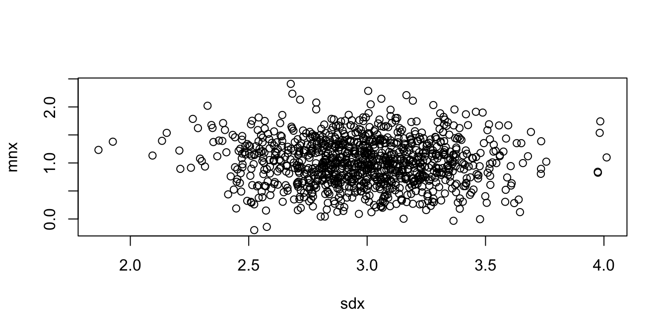

FIGURE F.76: Sample means and sample variances.

cor(mnx, sdx)
#> [1] -0.04240441

Exercise 12.26. We seek $c$ such that $\Pr(X \le c) = 0.90$ where $X\sim\chi^2(12)$. In R:

qchisq(0.9, df = 12)
#> [1] 18.54935

About 90% of the distribution lies below 18.549.

Exercise 12.27. By Theorem 12.10, $9 S^2 / 5 \sim \chi^2_9$, so \[ \Pr(S^2 > 10) = \Pr\!\left(\frac{9S^2}{5} > 18\right) = \Pr(\chi^2_9 > 18). \] In R:

pchisq(18, df = 9, lower.tail = FALSE)
#> [1] 0.03517354

Hence $\Pr(S^2 > 10) \approx 0.035$.

Exercise 12.28.

pop <- c(1, 3, 5, 7, 9)

# 1. Population mean and variance
mu    <- mean(pop)
sigma2 <- mean((pop - mu)^2)   # population variance (divide by N)
mu
#> [1] 5
sigma2
#> [1] 8

# 2. All samples of size 2 without replacement
samples <- combn(pop, 2)
samples
#>      [,1] [,2] [,3] [,4] [,5] [,6] [,7] [,8] [,9] [,10]
#> [1,]    1    1    1    1    3    3    3    5    5     7
#> [2,]    3    5    7    9    5    7    9    7    9     9

# 3. Sample mean for each
xbar <- apply(samples, 2, mean)
xbar
#>  [1] 2 3 4 5 4 5 6 6 7 8

# Mean and variance of sampling distribution
mean(xbar)
#> [1] 5
var_xbar <- mean((xbar - mean(xbar))^2)   # population variance of xbar
var_xbar
#> [1] 3

# 4. Verify E[Xbar] = mu
mean(xbar) == mu    # should be TRUE (or very close)
#> [1] TRUE

# 5. Relationship: var(Xbar) should equal sigma^2 * (N-n) / (n*(N-1))
# (finite population correction)
# For large populations, approximately sigma^2 / n
sigma2 / 2
#> [1] 4

The mean of the sampling distribution equals the population mean $\mu = 5$, confirming that $\overline{X}$ is an unbiased estimator of $\mu$. The variance of the sampling distribution is smaller than $\sigma^2$, and decreases as $n$ increases.

Exercise 12.29.

For Poisson($\lambda = 3$): $\operatorname{E}[X_i] = 3$; $\operatorname{var}[X_i] = 3$.
Algebraic argument: $\operatorname{E}[\overline{X}] = (1/n) \times \sum \operatorname{E}[X_i] = (1/n)\times n\times \lambda = \lambda$.

# 3. Simulation
set.seed(1)
lambda <- 3; n      <- 20; nsim   <- 10000

xbars <- replicate(nsim, mean(rpois(n, lambda)))
mean(xbars)   # should be close to 3
#> [1] 2.99858

# 4. Histogram
hist(xbars,
     main = "Sampling distribution of sample mean\nPoisson(3), n = 20",
     xlab = expression(bar(X)),
     freq = FALSE)
curve(dnorm(x, mean = lambda, sd = sqrt(lambda / n)),
      add = TRUE, lwd = 2)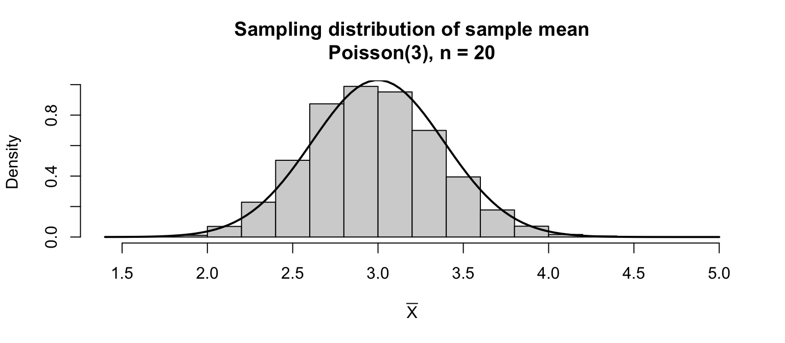

FIGURE F.77: A sampling distribution.

The average of the sample means is very close to $\lambda = 3$, confirming unbiasedness. The histogram is approximately bell-shaped, consistent with the Central Limit Theorem.

Exercise 12.30.

set.seed(2)
mu     <- 10; sigma2 <- 4; nsim   <- 10000

# Function for biased estimator
s2n <- function(x) sum((x - mean(x))^2) / length(x)

# n = 5
n <- 5
sims <- replicate(nsim, {
  x <- rnorm(n, mu, sqrt(sigma2))
  c(s2n(x), var(x))
})
cat("n = 5\n")
#> n = 5
cat("Mean of S2_n (biased):", mean(sims[1, ]), "\n")
#> Mean of S2_n (biased): 3.219432
cat("Mean of S2 (unbiased):", mean(sims[2, ]), "\n")
#> Mean of S2 (unbiased): 4.02429
cat("True sigma^2:", sigma2, "\n\n")
#> True sigma^2: 4

# n = 50
n <- 50
sims2 <- replicate(nsim, {
  x <- rnorm(n, mu, sqrt(sigma2))
  c(s2n(x), var(x))
})
cat("n = 50\n")
#> n = 50
cat("Mean of S2_n (biased):", mean(sims2[1, ]), "\n")
#> Mean of S2_n (biased): 3.915627
cat("Mean of S2 (unbiased):", mean(sims2[2, ]), "\n")
#> Mean of S2 (unbiased): 3.995538
cat("True sigma^2:", sigma2, "\n")
#> True sigma^2: 4

For $n = 5$, $S^2_n$ averages around $3.2 \approx (4/5)\times 4$, confirming bias. $S^2$ averages close to $4$, confirming unbiasedness. For $n = 50$ the bias of $S^2_n$ is much smaller, since $\operatorname{E}[S^2_n] = \frac{n - 1}{n}\sigma^2 \to \sigma^2$ as $n \to \infty$.

Exercise 12.31.

set.seed(3)
lambda <- 0.5   # rate; E[X] = 1/lambda = 2, var[X] = 1/lambda^2 = 4
nsim   <- 10000

# Theoretical values
mu_X    <- 1 / lambda; var_X   <- 1 / lambda^2

# n = 16
n <- 16
xbars16 <- replicate(nsim, mean(rexp(n, rate = lambda)))
cat("n = 16\n")
#> n = 16
cat("Theoretical mean of Xbar:", mu_X, "\n")
#> Theoretical mean of Xbar: 2
cat("Empirical  mean of Xbar:", mean(xbars16), "\n")
#> Empirical  mean of Xbar: 1.996384
cat("Theoretical var  of Xbar:", var_X / n, "\n")
#> Theoretical var  of Xbar: 0.25
cat("Empirical  var  of Xbar:", var(xbars16), "\n\n")
#> Empirical  var  of Xbar: 0.2557135

# n = 64
n <- 64
xbars64 <- replicate(nsim, mean(rexp(n, rate = lambda)))
cat("n = 64\n")
#> n = 64
cat("Theoretical var  of Xbar:", var_X / n, "\n")
#> Theoretical var  of Xbar: 0.0625
cat("Empirical  var  of Xbar:", var(xbars64), "\n")
#> Empirical  var  of Xbar: 0.06168541

As $n$ increases from $16$ to $64$ (fourfold), the variance of $\overline{X}$ decreases by a factor of four, consistent with $\operatorname{var}[\overline{X}] = \sigma^2/n$.

Exercise 12.32.

set.seed(4)
nsim <- 10000; mu_u  <- 0.5; var_u <- 1/12

par(mfrow = c(2, 2))
for (n in c(1, 5, 30, 100)) {
  xbars <- replicate(nsim, mean(runif(n)))
  hist(xbars,
       freq  = FALSE, xlim  = c(0, 1),
       main  = paste0("n = ", n),
       xlab  = expression(bar(X)))
  curve(dnorm(x, mu_u, sqrt(var_u / n)),
        add = TRUE, lwd = 2)
}

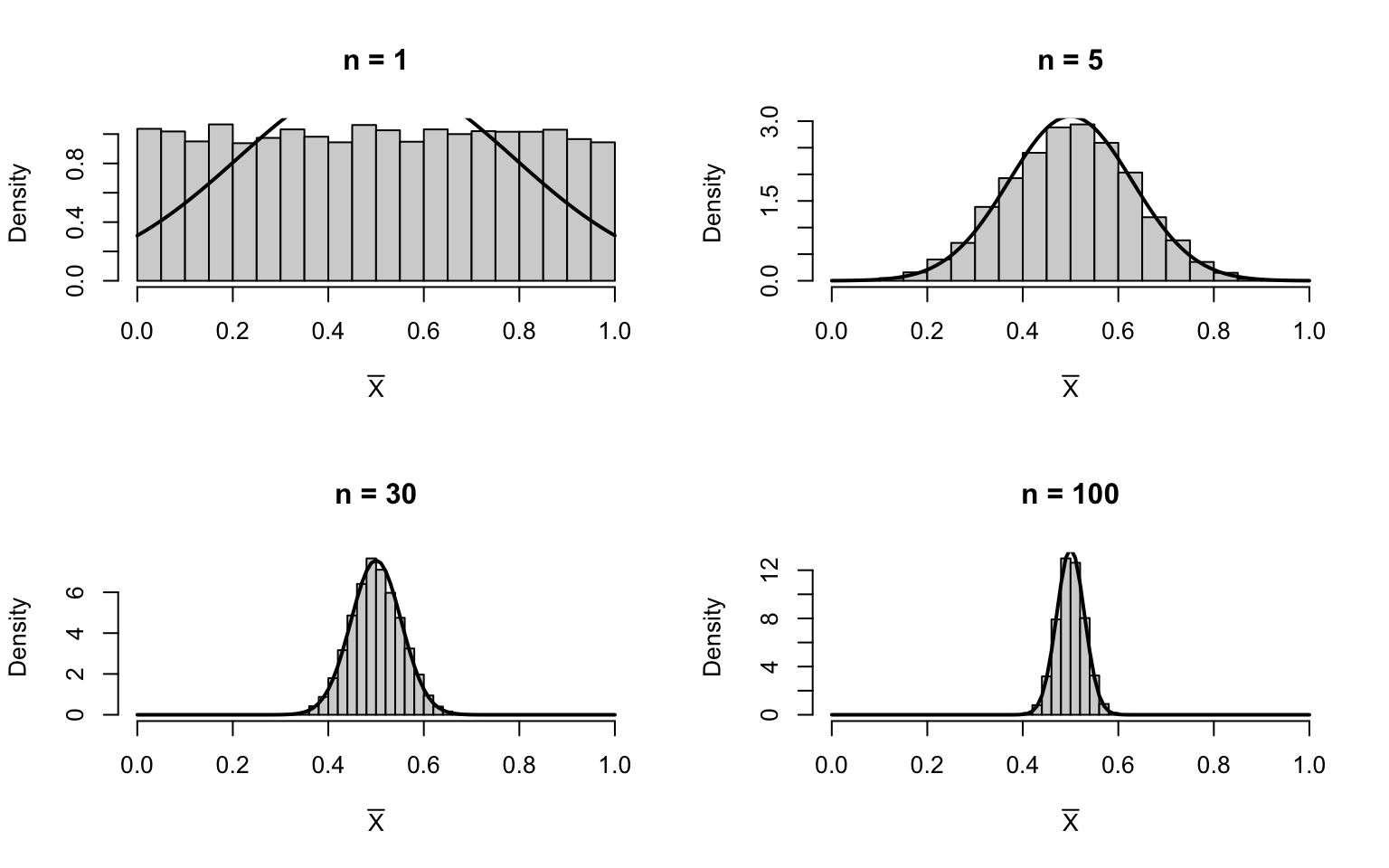
FIGURE F.78: Two estimates.

par(mfrow = c(1, 1))

For $n = 1$ the distribution is uniform. By $n = 5$ it is already roughly bell-shaped. By $n = 30$ it is closely approximated by the normal, and by $n = 100$ the approximation is excellent. The uniform distribution is symmetric, so convergence to normality is fast.

Exercise 12.33.

Total $T$ is the sum of $n$ Poisson($4$) rvs; $\text{Poisson}(n\times \lambda) = \text{Poisson}(200)$; $\operatorname{E}[T] = 200$; $\operatorname{var}[T] = 200$.

lambda <- 4; n <- 50

# 2. Normal approximation: T ~ N(200, 200)
mu_T  <- n * lambda
sd_T  <- sqrt(n * lambda)
prob_approx <- 1 - pnorm(215, mean = mu_T, sd = sd_T)
cat("Normal approximation Pr(T > 215):", prob_approx, "\n")
#> Normal approximation Pr(T > 215): 0.1444222

# 3. Exact probability using Poisson
prob_exact <- 1 - ppois(215, lambda = n * lambda)
cat("Exact Poisson    Pr(T > 215):", prob_exact, "\n")
#> Exact Poisson    Pr(T > 215): 0.1369904

The normal approximation is close to the exact Poisson probability. With $n = 50$ and $\lambda = 4$, the CLT provides a good approximation.

Exercise 12.34.

mu <- 500; sigma <- 8

# 1. P(X < 490) for a single item
p1 <- pnorm(490, mean = mu, sd = sigma)
cat("P(single item < 490):", p1, "\n")
#> P(single item < 490): 0.1056498

# 2. P(Xbar < 490) for n = 25
p2 <- pnorm(490, mean = mu, sd = sigma / sqrt(25))
cat("P(Xbar < 490), n = 25:", p2, "\n")
#> P(Xbar < 490), n = 25: 2.052263e-10

# 3. P(Xbar < 490) for n = 64
p3 <- pnorm(490, mean = mu, sd = sigma / sqrt(64))
cat("P(Xbar < 490), n = 64:", p3, "\n")
#> P(Xbar < 490), n = 64: 7.619853e-24

As $n$ increases, $\operatorname{var}[\overline{X}] = \sigma^2/n$ decreases, so the distribution of $\overline{X}$ becomes more concentrated around $\mu = 500$. Values far from the mean, like $490$, become increasingly unlikely.

Exercise 12.35.

# 1. E[Y] = 3*5 - 2*2 = 11; var[Y] = 9*9 + 4*4 = 81 + 16 = 97
E_Y   <- 3*5 - 2*2
var_Y <- 3^2 * 9 + (-2)^2 * 4
cat("E[Y]   =", E_Y, "\n")
#> E[Y]   = 11
cat("var[Y] =", var_Y, "\n")
#> var[Y] = 97

# 2. Y ~ N(11, 97)

# 3. P(Y > 20)
p <- 1 - pnorm(20, mean = E_Y, sd = sqrt(var_Y))
cat("P(Y > 20) =", p, "\n")
#> P(Y > 20) = 0.1804079

# 4. Simulation
set.seed(5)
nsim <- 50000
X1 <- rnorm(nsim, 5, 3); X2 <- rnorm(nsim, 2, 2)
Y  <-  3*X1 - 2*X2
cat("Simulated P(Y > 20):", mean(Y > 20), "\n")
#> Simulated P(Y > 20): 0.1821

$Y \sim N(11, 97)$. The theoretical and simulated probabilities agree closely.

Exercise 12.36.

$\operatorname{E}[X] = 10$; $\operatorname{var}[X] = 20$ (for $\chi^2_{10}$).

# 2. P(X < 15.99)
pchisq(15.99, df = 10)
#> [1] 0.900081

# 3. x such that P(X > x) = 0.05
qchisq(0.95, df = 10)
#> [1] 18.30704

# 4. Simulation and histogram
set.seed(6)
x_sim <- rchisq(10000, df = 10)
hist(x_sim,
     freq   = FALSE,
     main   = "Chi-squared (df = 10)",
     xlab   = expression(italic(x)))
curve(dchisq(x, df = 10), add = TRUE, lwd = 2)
legend("topright", legend = "Theoretical density",
       lwd = 2, bty = "n")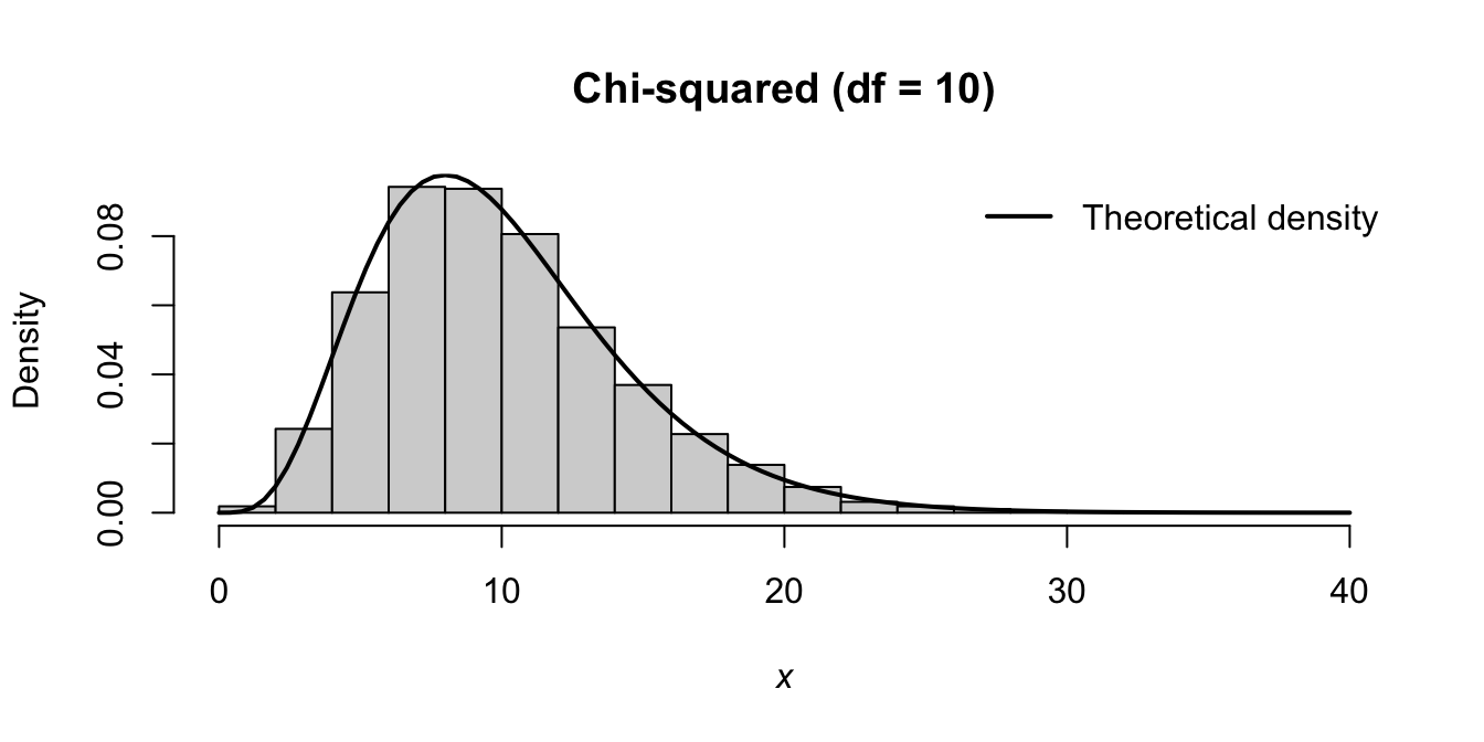

FIGURE F.79: A chi-squared distribution.

The histogram matches the theoretical $\chi^2_{10}$ density closely.

Exercise 12.37.

set.seed(7)
nsim <- 10000; n    <- 5

# 1. Simulate sum of 5 squared standard normals
chi_sim <- replicate(nsim, sum(rnorm(n)^2))

hist(chi_sim,
     freq   = FALSE,
     main   = expression(Sum~of~5~squared~N(0,1)~variates),
     xlab   = expression(sum(Z[i]^2, i==1, 5)) )
curve(dchisq(x, df = n), add = TRUE, lwd = 2)
legend("topright", legend = expression(chi[5]^2~density),
       lwd = 2, bty = "n")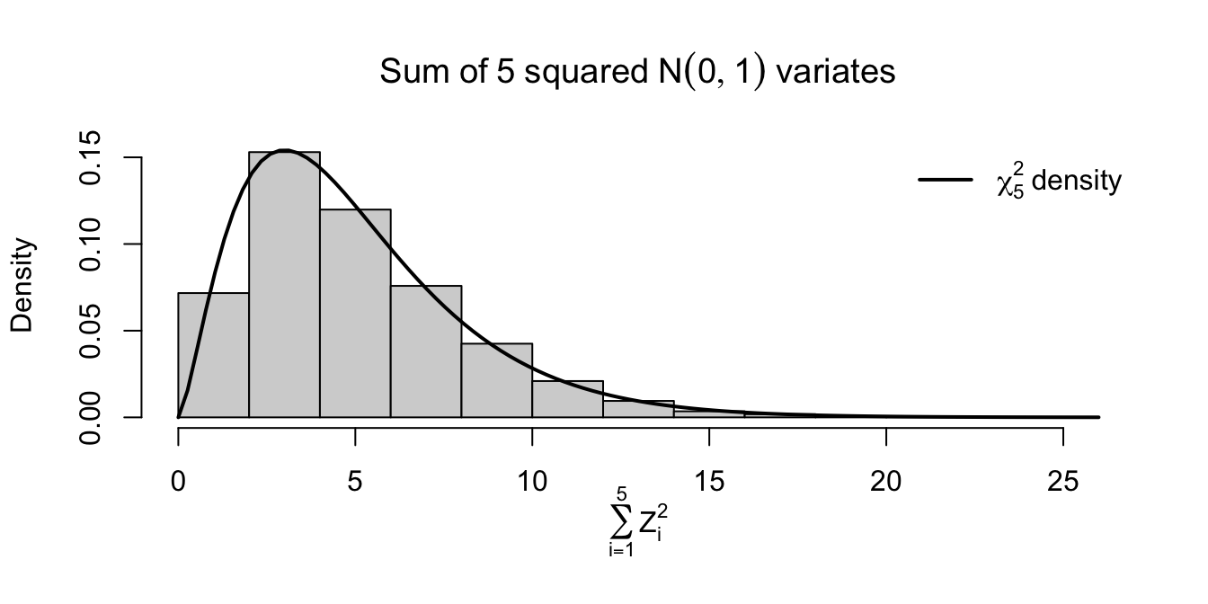

FIGURE F.80: Two estimates.


# 2. Empirical vs theoretical mean and variance
cat("Empirical mean:", mean(chi_sim), "  Theoretical:", n, "\n")
#> Empirical mean: 5.015286   Theoretical: 5
cat("Empirical var: ", var(chi_sim),  "  Theoretical:", 2*n, "\n")
#> Empirical var:  9.753725   Theoretical: 10

The histogram closely follows the $\chi^2_5$ density, confirming that the sum of $n$ squared standard normal variates follows a $\chi^2_n$ distribution.

Exercise 12.38.

$(n - 1)S^2 / \sigma^2 \sim \chi^2_{n - 1} = \chi^2_{14}$.

n <- 15; mu <- 2; sigma2 <- 9

# 2. P(S^2 > 14)
# Equivalent to P(chi^2_14 > (n-1)*14/sigma^2)
val <- (n - 1) * 14 / sigma2
p_exact <- 1 - pchisq(val, df = n - 1)
cat("P(S^2 > 14):", p_exact, "\n")
#> P(S^2 > 14): 0.08329722

# 3. s^2 such that P(S^2 > s^2) = 0.10
chi_crit <- qchisq(0.90, df = n - 1)
s2_crit  <- chi_crit * sigma2 / (n - 1)
cat("s^2 such that P(S^2 > s^2) = 0.10:", s2_crit, "\n")
#> s^2 such that P(S^2 > s^2) = 0.10: 13.54124

# 4. Simulation verification
set.seed(8)
nsim   <- 10000
s2_sim <- replicate(nsim, var(rnorm(n, mu, sqrt(sigma2))))
cat("Simulated P(S^2 > 14):", mean(s2_sim > 14), "\n")
#> Simulated P(S^2 > 14): 0.0816

The simulated probability matches the theoretical value closely.

Exercise 12.39.

# 1. E[T] = 0 (nu > 1); var[T] = nu/(nu-2) = 8/6 = 4/3
cat("E[T]   =", 0, "\n")
#> E[T]   = 0
cat("var[T] =", 8/6, "\n")
#> var[T] = 1.333333

# 2. P(T < 1.86) for t_8
pt(1.86, df = 8)
#> [1] 0.9500347

# 3. t such that P(|T| > t) = 0.05
qt(0.975, df = 8)
#> [1] 2.306004

# 4. Simulation
set.seed(9)
nsim  <- 20000
Z     <- rnorm(nsim)
V     <- rchisq(nsim, df = 8)
T_sim <- Z / sqrt(V / 8)

hist(T_sim,
     freq   = FALSE, breaks = 60, xlim   = c(-6, 6),
     main   = "Simulated t distribution (df = 8)",
     xlab   = expression(italic(T)))
curve(dt(x, df = 8),
      add = TRUE, lwd = 2)
legend("topright", legend = expression(t[8]~density),
       lwd = 2, bty = "n")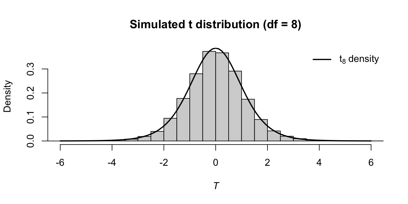

FIGURE F.81: A simulated $t$-distribution.

The simulated distribution aligns closely with the $t_8$ density, confirming the definition.

Exercise 12.40.

x <- c(14.2, 15.8, 13.5, 16.1, 14.9, 15.3, 13.8, 16.4, 14.6, 15.0)
n <- length(x)
mu0 <- 15

# 1. Sample mean and variance
xbar <- mean(x)
s2   <- var(x)
cat("Sample mean:", xbar, "\n")
#> Sample mean: 14.96
cat("Sample variance:", s2, "\n")
#> Sample variance: 0.9315556

# 2. T statistic
T_stat <- (xbar - mu0) / (sqrt(s2) / sqrt(n))
cat("T statistic:", T_stat, "\n")
#> T statistic: -0.1310556

# 3. Two-sided p-value
p_val <- 2 * pt(-abs(T_stat), df = n - 1)
cat("Two-sided p-value:", p_val, "\n")
#> Two-sided p-value: 0.8986141

The $T$-statistic is close to zero and the two-sided $p$-value is large, indicating no strong evidence against $\mu = 15$. The data are consistent with a population mean of $15$.

Exercise 12.41.

# 1. E[X] = nu2/(nu2-2) = 20/18 = 10/9
#    var[X] = 2*nu2^2*(nu1+nu2-2) / (nu1*(nu2-2)^2*(nu2-4))
nu1 <- 4; nu2 <- 20
E_X   <- nu2 / (nu2 - 2)
var_X <- 2 * nu2^2 * (nu1 + nu2 - 2) / (nu1 * (nu2-2)^2 * (nu2-4))
cat("E[X]   =", E_X, "\n")
#> E[X]   = 1.111111
cat("var[X] =", var_X, "\n")
#> var[X] = 0.8487654

# 2. P(X < 2.87)
pf(2.87, df1 = nu1, df2 = nu2)
#> [1] 0.9502145

# 3. x such that P(X > x) = 0.01
qf(0.99, df1 = nu1, df2 = nu2)
#> [1] 4.43069

# 4. Simulation
set.seed(10)
nsim  <- 20000
U1    <- rchisq(nsim, df = nu1)
U2    <- rchisq(nsim, df = nu2)
F_sim <- (U1 / nu1) / (U2 / nu2)

hist(F_sim,
     freq   = FALSE, breaks = 80, xlim   = c(0, 8),
     main   = expression(Simulated~F[4*","*20]~distribution),
     xlab   = expression(italic(F)))
curve(df(x, df1 = nu1, df2 = nu2),
      add = TRUE, lwd = 2)
legend("topright", legend = expression(F[4*","*20]~density),
       lwd = 2, bty = "n")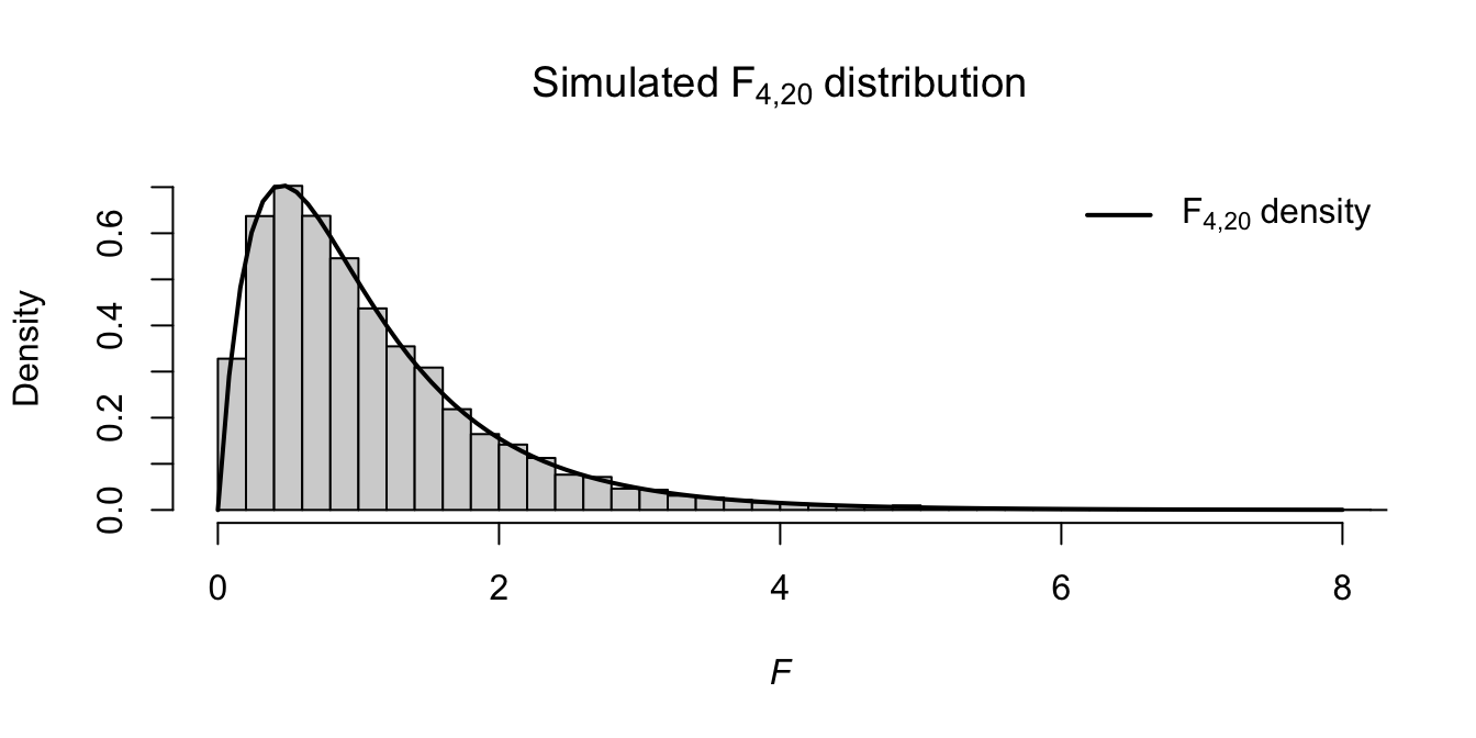

FIGURE F.82: An $F$-distribution..

The simulated ratio matches the $F_{4,20}$ density, confirming the relationship between chi-squared variates and the $F$-distribution.

Exercise 12.42.

If $T\sim t_n$, then $T^2 \sim F_{1, n}$.

# 2. P(T^2 > 3) using t_12
#    T^2 > 3 iff |T| > sqrt(3)
p_t <- 2 * pt(-sqrt(3), df = 12)
cat("P(T^2 > 3) via t_12:", p_t, "\n")
#> P(T^2 > 3) via t_12: 0.1088643

# 3. Equivalent via F_{1,12}
p_f <- 1 - pf(3, df1 = 1, df2 = 12)
cat("P(F > 3) via F_{1,12}:", p_f, "\n")
#> P(F > 3) via F_{1,12}: 0.1088643

# 4. Simulation comparison
set.seed(11)
nsim   <- 50000
T_sims <- rt(nsim, df = 12)
W_sims <- rf(nsim, df1 = 1, df2 = 12)

par(mfrow = c(1, 2))
hist(T_sims^2,
     freq   = FALSE, breaks = 80, xlim   = c(0, 15),
     main   = expression(T^2~where~T%~%t[12]),
     xlab   = expression(T^2))
curve(df(x, 1, 12), add = TRUE, lwd = 2)

hist(W_sims,
     freq   = FALSE, breaks = 80, xlim   = c(0, 15),
     main   = expression(W%~%F[1*","*12]),
     xlab   = expression(italic(W)) )
curve(df(x, 1, 12), add = TRUE, lwd = 2)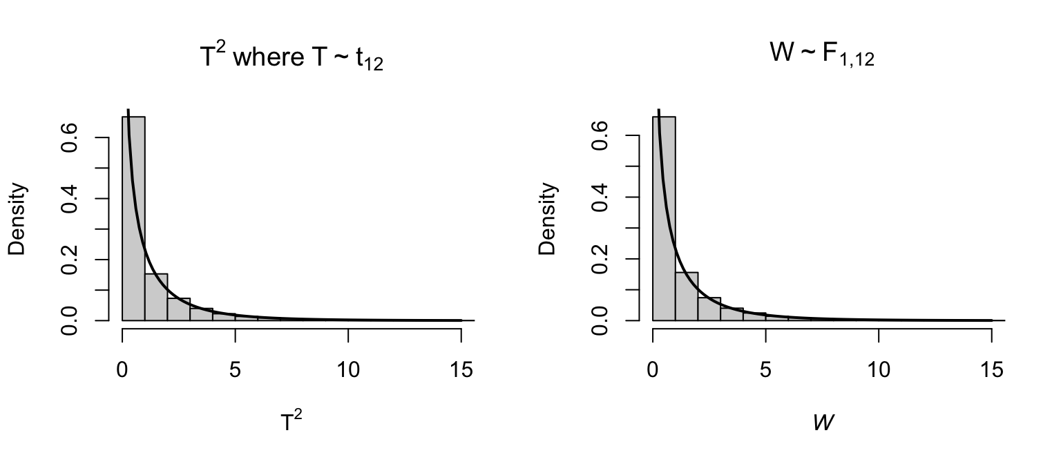

FIGURE F.83: Two distributions.

par(mfrow = c(1, 1))

The two probabilities are equal, and the histograms are visually identical, confirming that $T^2 \sim F_{1,12}$ when $T \sim t_{12}$.

Exercise 12.43.

Exact distribution: $Y \sim \text{Binomial}(120, 0.35)$.

p <- 0.35; n <- 120

# 2. Approximate: Y ~ N(np, np(1-p)) = N(42, 27.3)
mu_Y  <- n * p
var_Y <- n * p * (1 - p)
cat("Approximate distribution: N(", mu_Y, ",", var_Y, ")\n")
#> Approximate distribution: N( 42 , 27.3 )

# 3. Normal approximation P(Y >= 50)
p_approx <- 1 - pnorm(49.5, mean = mu_Y, sd = sqrt(var_Y))  # continuity correction
cat("Normal approximation P(Y >= 50):", p_approx, "\n")
#> Normal approximation P(Y >= 50): 0.07558328

# Without continuity correction
p_approx2 <- 1 - pnorm(50, mean = mu_Y, sd = sqrt(var_Y))
cat("Without continuity correction:  ", p_approx2, "\n")
#> Without continuity correction:   0.06287012

# 4. Exact binomial
p_exact <- 1 - pbinom(49, size = n, prob = p)
cat("Exact binomial P(Y >= 50):      ", p_exact, "\n")
#> Exact binomial P(Y >= 50):       0.07682402

The normal approximation with continuity correction is close to the exact binomial probability. Without the correction there is slightly more error.

Exercise 12.44.

set.seed(12)
nsim <- 5000; n    <- 30

results <- replicate(nsim, {
  x <- rnorm(n, mean = 0, sd = 1)
  c(mean(x), var(x))
})

xbars <- results[1, ]
s2s   <- results[2, ]

# 1. Scatterplot
plot(xbars, s2s,
     pch  = ".",
     main = "Sample mean vs sample variance\nfrom N(0,1), n = 30",
     xlab = expression(bar(X)),
     ylab = expression(S^2))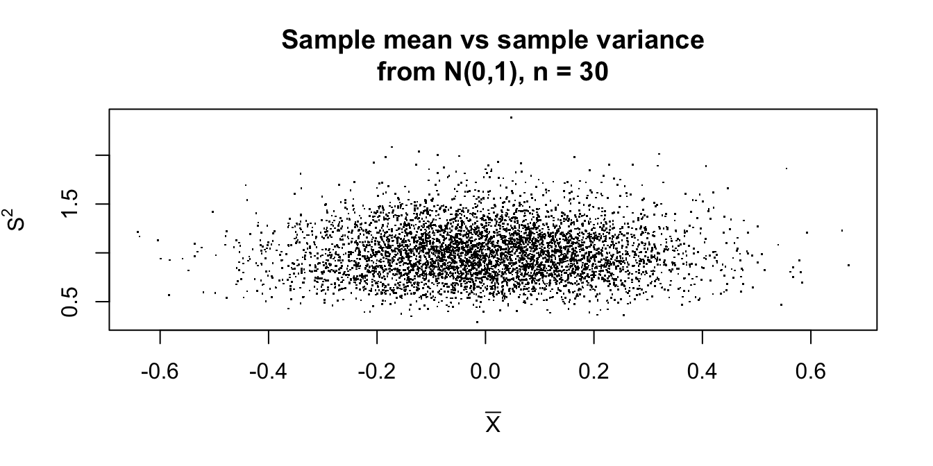

FIGURE F.84: Correlations between sample mean and sample variance.


# 2. Correlation
r <- cor(xbars, s2s)
cat("Correlation between Xbar and S^2:", round(r, 4), "\n")
#> Correlation between Xbar and S^2: 0.0093

The scatterplot shows no discernible pattern and the correlation is very close to zero, consistent with the theoretical result that $\overline{X}$ and $S^2$ are independent when sampling from a normal distribution.

Exercise 12.45.

Using $X_i - \overline{X} = (X_i - \mu) - (\overline{X} - \mu)$, we have \[\begin{align*} \sum_{i=1}^n (X_i - \overline{X})^2 &= \sum_{i=1}^n \left[(X_i - \mu) - (\overline{X} - \mu)\right]^2 \\ &= \sum_{i=1}^n \left[(X_i - \mu)^2 - 2(X_i - \mu)(\overline{X} - \mu) + (\overline{X} - \mu)^2\right]. \end{align*}\] Now distribute the summation: \[\begin{align*} \sum_{i=1}^n (X_i - \overline{X})^2 &= \sum_{i=1}^n (X_i - \mu)^2 - 2(\overline{X} - \mu)\sum_{i=1}^n (X_i - \mu) + \sum_{i=1}^n (\overline{X} - \mu)^2. \end{align*}\] Since $\sum_{i=1}^n (X_i - \mu) = n(\overline{X} - \mu)$, and $(\overline{X} - \mu)^2$ does not depend on $i$, \[ \sum_{i=1}^n (\overline{X} - \mu)^2 = n(\overline{X} - \mu)^2. \] Therefore, \[\begin{align*} \sum_{i=1}^n (X_i - \overline{X})^2 &= \sum_{i=1}^n (X_i - \mu)^2 - 2n(\overline{X} - \mu)^2 + n(\overline{X} - \mu)^2 \\ &= \sum_{i=1}^n (X_i - \mu)^2 - n(\overline{X} - \mu)^2. \end{align*}\]

Exercise 12.46.

For $X_i \sim \text{Uniform}(0,\theta)$, $\operatorname{E}[X_i] = \theta/2$, so $\operatorname{E}[2\overline{X}] = 2 \cdot \theta/2 = \theta$. Hence $\hat{\theta} = 2\overline{X}$ is unbiased.
\[ \operatorname{Bias}(\tilde{\theta}) = \frac{n}{n+1}\theta - \theta = -\frac{\theta}{n+1} < 0. \] The estimator underestimates $\theta$: the largest observed value cannot exceed $\theta$, so $\tilde\theta$ is always below the true upper bound.
\[ \operatorname{E}\!\left[\frac{n+1}{n}\tilde{\theta}\right] = \frac{n+1}{n} \cdot \frac{n}{n+1}\theta = \theta. \] So $\frac{n + 1}{n}\max(X_1,\dots, X_n)$ is unbiased.
See R code below. Both estimators should be approximately unbiased (means close to $\theta = 5$), but the adjusted maximum has smaller variance than $2\overline{X}$, illustrating that unbiasedness alone does not determine which estimator is preferable.
The adjusted $\tilde{\theta}$ uses the most extreme observation, which carries the most information about $\theta$ in a uniform distribution. For large $n$, $\max(X_1,\dots, X_n)$ is very close to $\theta$, so the adjusted estimator becomes very precise. By contrast, $2\overline{X}$ averages out information across all observations and remains comparatively noisy.

set.seed(42)
theta <- 5;  n <- 10;  B <- 10000

samples <- matrix(runif(B * n, min = 0, max = theta), nrow = B, ncol = n)

theta_hat   <- 2 * rowMeans(samples)                        # 2 * x-bar
theta_tilde <- (n + 1) / n * apply(samples, 1, max)         # adjusted maximum

# Bias (both should be near zero)
mean(theta_hat)   - theta
#> [1] 0.007077966
mean(theta_tilde) - theta
#> [1] 0.006389918

# Variability
var(theta_hat)
#> [1] 0.8318727
var(theta_tilde)
#> [1] 0.2005911

# Visual comparison
par(mfrow = c(1, 2))
hist(theta_hat,   breaks = 50, main = expression(2 * bar(X)),
     xlab = expression(hat(theta)) )
abline(v = theta, col = "grey", lty = 2, lwd = 2)

hist(theta_tilde, breaks = 50, 
     main = expression(frac(n + 1, n) * max(X[1], ldots, X[n])),
     xlab = expression(tilde(theta)) )
abline(v = theta, lty = 2, lwd = 2)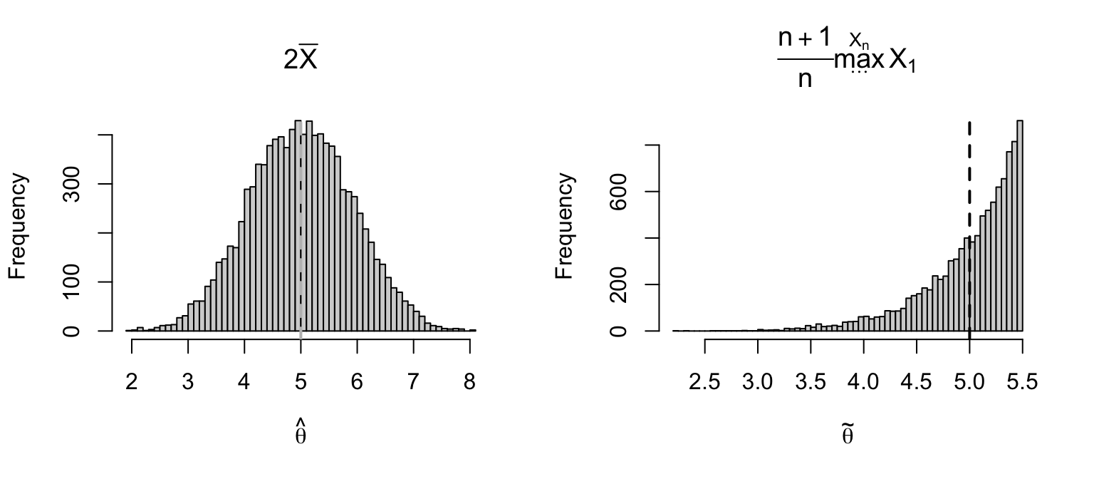

FIGURE F.85: Two estimates.

Exercise 12.47.

Solve $F_X(x) = 1.2$: $1 - \exp(-\lambda x)$ gives $M = \ln(2)/\lambda$.
Since $X_i \sim \text{Exponential}(\lambda)$, we have $\operatorname{E}[X_i] = 1/\lambda$, and so $\operatorname{E}[\overline{X}] = 1/\lambda$.
The bias is \[ \operatorname{Bias}(\widehat{M}) = \operatorname{E}[\overline{X}] - M = \frac{1}{\lambda} - \frac{\ln 2}{\lambda} = \frac{1 - \ln 2}{\lambda} > 0. \] Since $\ln 2 \approx 0.693 < 1$, the bias is positive: $\overline{X}$ systematically overestimates the median.
Define $\tilde{M} = \ln(2)\,\overline{X}$. Then \[ \operatorname{E}[\tilde{M}] = \ln(2)\operatorname{E}[\overline{X}] = \frac{\ln 2}{\lambda} = M, \] so $\tilde{M} = \ln(2)\,\overline{X}$ is an unbiased estimator of the median.

Exercise 12.48.

See R below. As $\nu$ increases, $P(T > 2)$ decreases toward the normal value.

$\nu$	$P(T > 2)$
5	0.0510
10	0.0367
30	0.0273
100	0.0233
$\infty$ (normal)	0.0228

Heavier tails means more probability is placed in the extremes relative to the normal distribution. For small $\nu$, $P(T > 2)$ is substantially larger than the corresponding normal probability, meaning extreme values are more likely under the $t$-distribution. This extra probability in the tails reflects the additional uncertainty from estimating $\sigma$.
See R below.

$\nu$	$t^*$
5	2.571
10	2.228
30	2.042
$\infty$ (normal)	1.960

As $\nu$ increases, $t^*$ decreases toward $1.96\approx 2$, the familiar normal percentage point. For small $\nu$ a wider interval is needed to capture the central $95\%$ of probability, again reflecting the heavier tails.

### PART 1
nu <- c(5, 10, 30, 100)
probs <- pt(2, df = nu, lower.tail = FALSE)
round(data.frame(nu = nu, P_T_gt_2 = probs), 4)
#>    nu P_T_gt_2
#> 1   5   0.0510
#> 2  10   0.0367
#> 3  30   0.0273
#> 4 100   0.0241
# Normal comparison
pnorm(2, lower.tail = FALSE)
#> [1] 0.02275013

### PART 3
nu <- c(5, 10, 30)
tstar <- qt(0.975, df = nu)
round(data.frame(nu = nu, tstar = tstar), 4)
#>   nu  tstar
#> 1  5 2.5706
#> 2 10 2.2281
#> 3 30 2.0423
qt(0.975, df = Inf)   # normal limit
#> [1] 1.959964

Exercise 12.49.

See R below. When both degrees of freedom are small the distribution is strongly right-skewed. As the degrees of freedom increase the distribution becomes more symmetric and concentrates around $1$, reflecting the fact that $F \to 1$ in probability as $\nu_1, \nu_2 \to \infty$.
By definition, if $U \sim \chi^2_{\nu_1}$ and $V \sim \chi^2_{\nu_2}$ are independent, then \[ F = \frac{U/\nu_1}{V/\nu_2} \sim F_{\nu_1,\nu_2} \quad\text{thus}\quad \frac{1}{F} = \frac{V/\nu_2}{U/\nu_1} \sim F_{\nu_2,\nu_1}, \] since the roles of $U$ and $V$ are simply exchanged.
\[ P(F_{\nu_1,\nu_2} \leq x) = P\!\left(\frac{1}{F_{\nu_1,\nu_2}} \geq \frac{1}{x}\right) = P\!\left(F_{\nu_2,\nu_1} \geq \frac{1}{x}\right), \] where the last step uses Part 2.
See R below.

### PART 1
x <- seq(0, 5, length.out = 500)
params <- list(c(5, 5), c(5, 30), c(30, 5), c(30, 30))
lty <- 1:4
plot(x, df(x, 5, 5), type = "l", lwd = 3, lty = lty,
     ylab = "Density", xlab = "x", main = "F distribution pdfs",
     ylim = c(0, 1.5))
for (i in 2:4) {
  lines(x, df(x, params[[i]][1], params[[i]][2]), 
        lty = lty[i], lwd = 2)
}
legend("topright", 
       legend = c("F(5,5)","F(5,30)","F(30,5)","F(30,30)"),
       lty = lty, lwd = 2)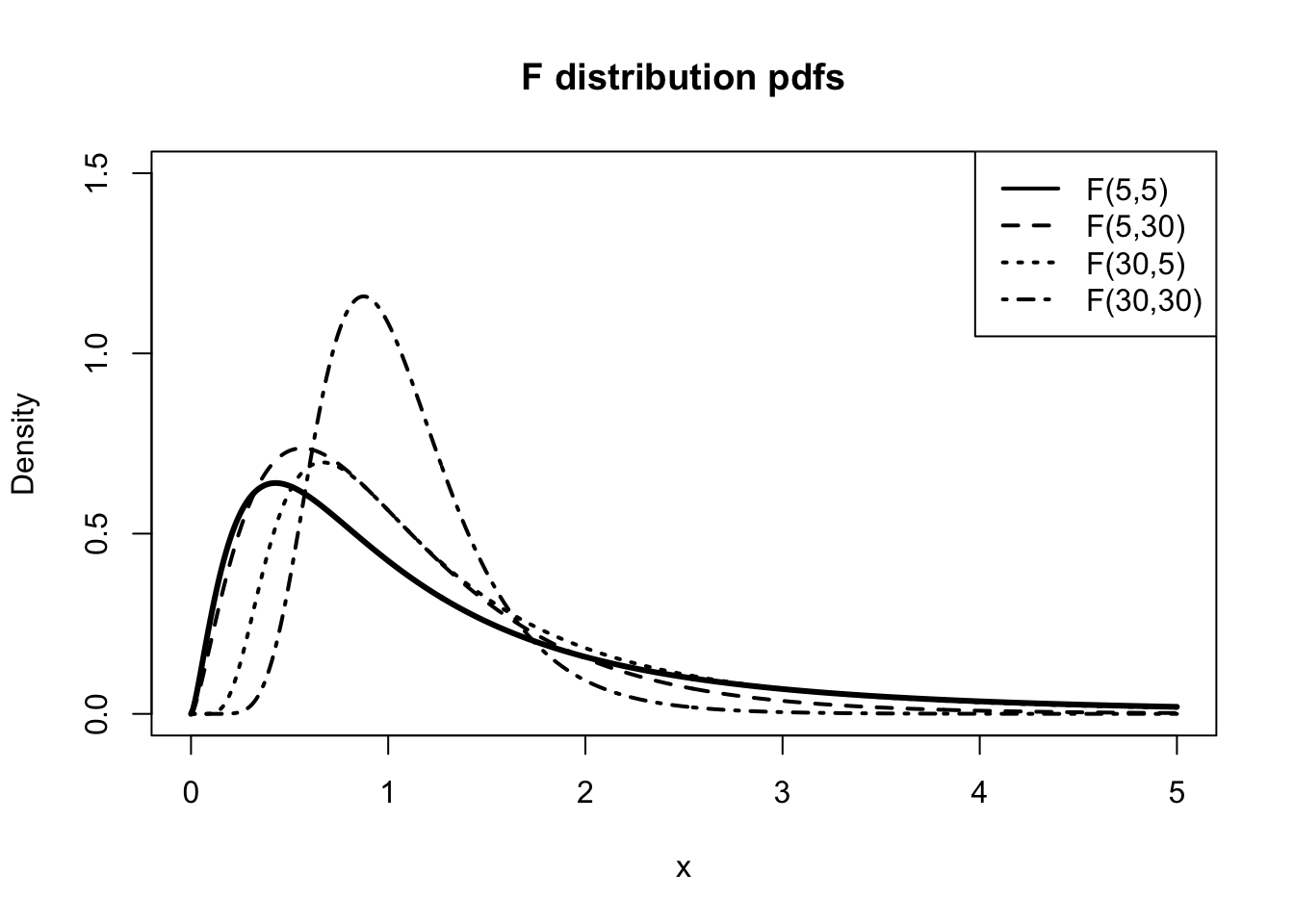


### PART 4
pf(0.4, df1 = 5, df2 = 10)                        # P(F_{5,10} <= 0.4)
#> [1] 0.1618347
pf(2.5, df1 = 10, df2 = 5, lower.tail = FALSE)     # P(F_{10,5} >= 2.5)
#> [1] 0.1618347
# Both should return the same value, approximately 0.1256

F.12 Answers for Chap. 13

Exercise 13.1. Compare the PDF in Eq. (13.1) to the beta distribution PDF.

Exercise 13.2. Compare the expressions for $\operatorname{E}[X]$ and $\operatorname{E}[X^2]$ to the beta distribution PDF.

Exercise 13.3. $\displaystyle \frac{n!}{(k - 1)!\,(n - k)!} \frac{(x + 1)^{k - 1} (1 - x)^{n - k}}{2^n}$ for $-1\le x\le 1$.

Exercise 13.4. $\displaystyle f_{(Y)}(y) = \frac{n!}{(k - 1)! (n - k)!} \frac{x^{2k - 1}}{2\, 4^{k - 1}}\left(1 - \frac{x^2}{4}\right)^{n - k}$ for $0 < x < 2$.

Exercise 13.10. Fix the initial draw: $X = x$. Given that value, each $Y_i \sim\text{Unif}(0, 1)$ is independent of the others, and the probability that $Y_i > x$ is $1 - x$. So for fixed $x$, the number of trials $N$ until the first $Y > x$ has a geometric distribution with success probability $p = 1 - x$, and therefore $\operatorname{E}[X] = 1 / (1 - x)$. To find the overall expected value, we integrate over all possible $x \in [0, 1]$: \[ \operatorname{E}[N] = \operatorname{E}[1/(1 - X)] = \int_0^1 \frac{1}{1 - x}\, dx, \] which diverges. Thus, $\operatorname{E}[N] = \infty$.

F.13 Answers for Chap. 14

Exercise 14.1.

$f(\theta| y)\propto f(y\mid\theta)\times f(\theta)$, where (given): \[ f(y\mid \theta) = (1 - \theta)^y\theta \quad\text{and}\quad f(\theta) = \frac{\theta^{m - 1}(1 - \theta)^{n - 1}}{B(m, n)}. \] Combining then: $f(\theta| y)\propto \theta^{(m + 1) - 1} (1 - \theta)^{(n + y) - 1}$. which is a beta distribution with parameters $m + 1$ and $n + y$.
Prior: $\operatorname{E}[\theta] = m / (m + n) = 1.2/(1.2 + 2) = 0.375$. So then, $\operatorname{E}[Y] = (1 - p)/p = 1.667$.
Posterior: $\operatorname{E}[\theta] = (m + 1)/(m + 1 + n + y) = 0.3056$; slightly reduced.

E Using R with distributions

G References

Cumulant	Formula
\(\kappa_1 = E[S]\)	\(\lambda\alpha/\beta\)
\(\kappa_2 = \text{var}[S]\)	\(\lambda\alpha(\alpha+1)/\beta^2\)
\(\kappa_3\)	\(\lambda\alpha(\alpha+1)(\alpha+2)/\beta^3\)
\(\kappa_4\)	\(\lambda\alpha(\alpha+1)(\alpha+2)(\alpha+3)/\beta^4\)

	\(Y_1 = 1\)	\(Y_1 = 2\)
\(Y_2 = 0\)	\(2/6\)	\(0\)
\(Y_2 = 1\)	\(1/6\)	\(3/6\)

	\(C = 0\)	\(C = 1\)
\(D = 0\)	\(6/36\)	\(6/36\)
\(D = 1\)	\(12/36\)	\(12/36\)

.	Die 1: 1	2	3	4	5	6
Die 2: 1	\((1, 1)\)	\((2, 1)\)	\((3, 1)\)	\((4, 1)\)	\((5, 1)\)	\((6, 1)\)
2	\((2, 1)\)	\((2, 2)\)	\((3, 2)\)	\((4, 2)\)	\((5, 2)\)	\((6, 2)\)
3	\((3, 1)\)	\((3, 2)\)	\((3, 3)\)	\((4, 3)\)	\((5, 3)\)	\((6, 3)\)
4	\((4, 1)\)	\((4, 2)\)	\((4, 3)\)	\((4, 4)\)	\((5, 4)\)	\((6, 4)\)
5	\((5, 1)\)	\((5, 2)\)	\((5, 3)\)	\((5, 4)\)	\((5, 5)\)	\((6, 5)\)
6	\((6, 1)\)	\((6, 2)\)	\((6, 3)\)	\((6, 4)\)	\((6, 5)\)	\((6, 6)\)

	\(\text{min} = 1\)	\(\text{min} = 2\)	\(\text{min} = 3\)	\(\text{min} = 4\)	\(\text{min} = 5\)	\(\text{min} = 6\)
\(\text{max} = 1\)	1/36	0/36	0/36	0/36	0/36	0/36
\(\text{max} = 2\)	2/36	1/36	0/36	0/36	0/36	0/36
\(\text{max} = 3\)	2/36	2/36	1/36	0/36	0/36	0/36
\(\text{max} = 4\)	2/36	2/36	2/36	1/36	0/36	0/36
\(\text{max} = 5\)	2/36	2/36	2/36	2/36	1/36	0/36
\(\text{max} = 6\)	2/36	2/36	2/36	2/36	2/36	1/36