D Short R introduction
D.1 General ideas
When you start R, you are presented with a prompt asking you enter an instruction:
>We do not show this prompt with the R code in this book, to enable any code that we show do be cut-and-paste directly into R and evaluated.
The > is how R prompts you to enter something for it to do.
R can be used a fancy calculator:
(-5 + 7) * 2
#> [1] 4
2 * pi * 3
#> [1] 18.84956
exp(-1)
#> [1] 0.3678794
sqrt( 9 ) * sin(3 * pi / 2)
#> [1] -3
The output begins with [1] to indicate the first item of output; sometimes, numerous values appear in the output (see Sect. D.4 for examples).
Spaces are not important to R, so these are all the same:
1 +                2
#> [1] 3
1          +  2
#> [1] 3
1+2
#> [1] 3
1 + 2
#> [1] 3
The last is better for human readability, so is recommended.
R also allows variables to be used, and values can be assigned to variables using = or the more traditional <- combination of characters.
Variables cannot start with a digit.
Radius = 2
Area = pi * Radius^2
Area
#> [1] 12.56637

side1 <- 2
side2 <- 4
hypot <- sqrt( side1^2 + side2^2 )
hypot
#> [1] 4.472136
The value of a variable is displayed by typing the variable name.
Comments can be added using # followed by text; any text following a # is ignored by R:
hourly_Wage <- 20  # Hourly wage, in $ per hr
hours_Worked <- 16 # Number of hours worked

# This all assumes no overtime rates!

weekly_Income <- hourly_Wage * hours_Worked # Income in dollar for the week
weekly_Income
#> [1] 320
In complete lines of instructions cause R to wait for the instruction to be completed.
For instance, suppose you type:
R will change the prompt from a > to +, indicating that you need to add more information to complete the command.
Once the command is complete, R evaluates the instruction:
sqrt(4
)
#> [1] 2
D.2 Using functions in R
R has thousands of functions to perform specific tasks. We have already seen two being used above:
-
sqrt()takes the square root of a given value. -
exp()find the value of \(\exp(x) = \exp x\) for some given value of \(x\). -
log()finds the logarithm of a function.
Functions, in general, can take more than one input.
Consider the function log().
We can type
log(100)
#> [1] 4.60517
If we look at the help for the log() function (by typing ?log), we see the usage is described like this:
Usage
log(x, base = exp(1))
That is, the function can take two inputs: one called x, and one called base.
The help information is starting that the default value of base, if it is not told otherwise, is assumed to be exp(1) (which is \(\exp(1)= \exp 1 = 2.71828\dots\)).
In other words, the default logarithm is the natural logarithm.
Since the command above (i.e., log(100)) only gave one input to the log() function, the value of the second input (i.e., base) uses the default value of exp(1).
That is, \(\log_e 100 = \ln 100 = 4.605\dots\).
To specify a different base, we can set the value of base explicitly:
log(100, 10)
#> [1] 2
The inputs are assumed by R to have been given in the order shown in the help; that is x = 100 and base = 10.
It is clearer, though, to name the value of the second input:
log(100, base = 10)
#> [1] 2
The value of the first input can be named also:
log(x = 100, base = 10)
#> [1] 2
When inputs are named, they can appear in any order:
log(base = 10, x = 100)
#> [1] 2
Some functions in R have many inputs. Some functions are collected into R packages that provide additional functionality.
D.3 General functions
-
seq()produces a sequence of integers:-
seq(1, 4)produces the list: \(1\), \(2\), \(3\), \(4\). -
seq(0, 10, by = 2)produces a list going up by two each time: \(0\), \(2\), \(4\), \(6\), \(8\), \(10\). -
seq(0, 10, length = 3)produces a list of length three: \(0\), \(5\), \(10\). - A colon can also be used in special cases:
3 : 7produces: \(3\), \(4\), \(5\), \(6\), \(7\).
-
-
c()is used to concatenate (join together) a series of values:-
c("fred", "martha")creates a vector with two text elements. -
c(1, 8, 3.14, -2)create a vector with four numerical elements.
-
-
cat()is often used to print information. -
matrix()is used to produces matrices (of \(2\)-dimensions):-
matrix(data = c(1, 2, 3, 4, 5, 6), byrow = TRUE, ncol = 3)produces the \(2\times 3\) array (i.e.,ncol = 3means the number of columns is \(3\)): \[ \left[ \begin{array}{ccc} 1 & 2 & 3\\ 4 & 5 & 6\\ \end{array} \right]. \]
-
matrix(data = c(1, 2, 3, 4, 5, 6),
       byrow = TRUE,
       ncol = 3)
#>      [,1] [,2] [,3]
#> [1,]    1    2    3
#> [2,] 4 5 6-
matrix(data = c(1, 2, 3, 4, 5, 6), bycol = TRUE, nrow = 2produces the \(2\times 3\) array (i.e.,nrow = 2means the number of rows is \(2\)): \[ \left[ \begin{array}{ccc} 1 & 3 & 5\\ 2 & 4 & 6\\ \end{array} \right]. \] -
numeric()creates a numeric vector.-
numeric(4)produces an empty vector of length \(4\).
-
-
array()produces matrix-like structure, but they can have many dimensions (not just two, likematrix())-
array( dim = c(2, 4))produces an empty \(2\times 4\) array. -
array( data = c(1, 2, 3, 4, 5, 6, 7, 8), dim = c(2, 2, 2))produces a \(2\times 2\times 2\) array:
-
array( data = c(1, 2, 3, 4, 5, 6, 7, 8), dim = c(2, 2, 2))
#> , , 1
#>
#>      [,1] [,2]
#> [1,]    1    3
#> [2,]    2    4
#>
#> , , 2
#>
#>      [,1] [,2]
#> [1,]    5    7
#> [2,] 6 8-
t()transposes a matrix or array:
A <- matrix( c(1, -2, -20, 3), ncol = 2)
A
#>      [,1] [,2]
#> [1,]    1  -20
#> [2,]   -2    3
t(A)
#>      [,1] [,2]
#> [1,]    1   -2
#> [2,]  -20    3
Logical comparisons in R are possible (using of == rather than =):
Days_Of_Week <- c("Mon", "Tues", "Wed", "Thurs", "Fri", "Sat", "Sun")
Hours_Sleep <- c(8, 8, 8, 8, 6, 6, 10)

Hours_Sleep == 8
#> [1]  TRUE  TRUE  TRUE  TRUE FALSE FALSE FALSE
Hours_Sleep > 8
#> [1] FALSE FALSE FALSE FALSE FALSE FALSE  TRUE
Hours_Sleep >= 8
#> [1]  TRUE  TRUE  TRUE  TRUE FALSE FALSE  TRUE

Hours_Sleep == 6 | Hours_Sleep == 10 # | means "OR"
#> [1] FALSE FALSE FALSE FALSE  TRUE  TRUE  TRUE

Hours_Sleep > 6 & Hours_Sleep < 10 # & means "AND"
#> [1]  TRUE  TRUE  TRUE  TRUE FALSE FALSE FALSE

which(Hours_Sleep == 8)
#> [1] 1 2 3 4
which(Hours_Sleep > 8)
#> [1] 7
which(Hours_Sleep >= 8)
#> [1] 1 2 3 4 7

which(Hours_Sleep == 6 | Hours_Sleep == 10 ) # | means "OR"
#> [1] 5 6 7

which(Hours_Sleep > 6 & Hours_Sleep < 10 ) # & means "AND"
#> [1] 1 2 3 4

Weekend <- Days_Of_Week == "Sat" | Days_Of_Week == "Sun"

Week_Day <- !Weekend # ! means "NOT"

Hours_Sleep[Week_Day]
#> [1] 8 8 8 8 6

Hours_Sleep[Weekend]
#> [1]  6 10


cat("These are the hours of sleep on weekdays:", Hours_Sleep[Week_Day], "\n")
#> These are the hours of sleep on weekdays: 8 8 8 8 6
   # \n  is used to create a new line.
Specific elements of a vector can be accessed using square brackets:
Hours_Sleep[1]
#> [1] 8
Hours_Sleep[3:5]
#> [1] 8 8 6

Hours_Sleep[Weekend]
#> [1]  6 10
D.4 Vector operations
R is a vectorised system; that is, operations work on all elements of a vector:
x <- 0 : 8   # x  is a vector
x
#> [1] 0 1 2 3 4 5 6 7 8
x + 3
#> [1]  3  4  5  6  7  8  9 10 11
2 * x
#> [1]  0  2  4  6  8 10 12 14 16

sqrt(x) # The square root function
#> [1] 0.000000 1.000000 1.414214 1.732051 2.000000 2.236068
#> [7] 2.449490 2.645751 2.828427
cos(x)  # The cosine function
#> [1]  1.0000000  0.5403023 -0.4161468 -0.9899925 -0.6536436
#> [6]  0.2836622  0.9601703  0.7539023 -0.1455000
exp( -x ) # The exponential function
#> [1] 1.0000000000 0.3678794412 0.1353352832 0.0497870684
#> [5] 0.0183156389 0.0067379470 0.0024787522 0.0009118820
#> [9] 0.0003354626
D.5 Statistical functions
Because R is primarily a statistical package and environment, all the basic statistical functions are available, including:
-
mean(): Find the mean of a sample of values. Example:mean( c(1, 2, 3, 4)). -
median(): Find the median of a sample of values. Example:median( c(1, 2, 3, 4)). -
sd(): Finds the standard deviation of a sample of values. Example:sd( c(1, 2, 3, 4)). -
var(): Finds the variance of a sample of values. Example:var( c(1, 2, 3, 4)). -
lm(): To fit a linear regression model:
x <- c(1, 2, 3, 4, 5)
y <- c(12, 10, 9, 7, 4)

out <- lm(y ~ x) # Read: 'y as a function of x'
coef(out)
#> (Intercept)           x
#>        14.1        -1.9
summary(out)
#>
#> Call:
#> lm(formula = y ~ x)
#>
#> Residuals:
#>    1    2    3    4    5
#> -0.2 -0.3  0.6  0.5 -0.6
#>
#> Coefficients:
#>             Estimate Std. Error t value Pr(>|t|)
#> (Intercept)  14.1000     0.6351  22.202  0.00020 ***
#> x            -1.9000     0.1915  -9.922  0.00218 **
#> ---
#> Signif. codes:  0 '***' 0.001 '**' 0.01 '*' 0.05 '.' 0.1 ' ' 1
#>
#> Residual standard error: 0.6055 on 3 degrees of freedom
#> Multiple R-squared:  0.9704, Adjusted R-squared:  0.9606
#> F-statistic: 98.45 on 1 and 3 DF,  p-value: 0.002178
D.6 Probability and counting functions
- the number of combinations of
nelements takenkat a time is found usingchoose(n, k). -
\(n!\) is given by
factorial(n). - the number of permutations of
nelements takenkat a time is found usingchoose(n, k) * factorial(k). - a list of all combinations of
nelements,mat a time, is given bycombn(x, m). -
\(\Gamma(x)\) is given by
gamma(x).
D.7 Plotting functions
Three systems exists for plotting in R, believe it or not. Here, we discuss the base system.
plot() is the basic function for plotting, with many options:
-
plot(x, y)andplot(y ~ x)both produce a scatterplot, withyon the vertical axis andxon the horizontal axis. -
plot(..., type = "l")plots with lines rather than points. -
plot(..., lwd = "3")plots with a line width thrice as thick. -
plot(..., xlab = "text", ylab = "Info")adds an label to the x and y axes respectively. -
plot(..., main = "Title")adds a main title to the plot. -
plot(..., col = "green")plots in green rather than the default (black).
plot() starts a new canvas every time it is called.
lines() and points() add lines and points respectively to an existing plot.
legend() adds a legend to an existing plot.
x <- seq(0, 4, length = 100)
y1 <- dexp(x, rate = 2) # Probability function for an exponential distn

plot(y1 ~ x,
     type = "l", # Use lines, not points
     lwd = 2, # Make lines a bit thicker
     xlab = "Values of x",
     ylab = "Probability function",
     main = "Probability function for\nexponential distribution",
      # NOTE: using  \n  adds a line break, and # is used for comments
     col = "red",
     las = 1, # Makes the axis labels all horizontal
     xlim = c(0, 4.5), # Changes the displayed limits of the x-axis
     ylim = c(0, 3) ) # Changes the displayed limits on the y-axis

y2 <- dexp(x, rate = 3)
lines( y2 ~ x, # ADD a line to existing point
       lwd = 2,
       col = "blue")

legend("topright", # The location
       lwd = 2,
       col = c("red", "blue"),
       legend = c("Rate = 2",
                  "Rate = 3")
       )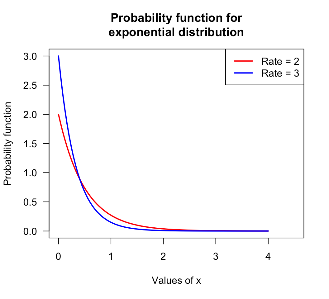
FIGURE D.1: An example plot: the probability function for two exponential distributions