9 Transformations of random variables

On completion of this chapter, you should be able to:

• derive the distribution of a transformed variable, given the distribution of the original variable, using the change of variable method.
• derive the distribution of a transformed variable, given the distribution of the original variable, using the distribution function method.
• derive the distribution of a transformed variable, given the distribution of the original variable, using the moment generating function method.

9.1 Introduction

In this chapter, we consider the distribution of a random variable \(Y = u(X)\), given a random variable \(X\) with known distribution, and a function \(u(\cdot)\). Among several available techniques, three are considered:

1. the change of variable method (Sect. 9.2);
2. the distribution function method (Sect. 9.3);
3. the moment generating function method (Sect. 9.4).

An important concept in this context is a one-to-one transformation.

Definition 9.1 (One-to-one transformation) Let \(Y = u(X)\), where the function \(u(\cdot)\) is defined on the range \(\mathcal{R}_X\) of the random variable \(X\). The transformation \(u(\cdot)\) is called a one-to-one transformation (or one-to-one mapping) on \(\mathcal{R}_X\) if distinct values of \(x\in\mathcal{R}_X\) produce distinct values of \(y\); that is, \[ u(x_1) = u(x_2)\implies x_1=x_2. \]

Equivalently, each \(y\in\mathcal{R}_Y\) corresponds to exactly one \(x\in\mathcal{R}_X\). We also write 1:1 transformation or 1:1 mapping.

When \(Y = u(X)\) is a one-to-one transformation on \(\mathcal{R}_X\), the inverse function \(u^{-1}\) is uniquely defined on \(\mathcal{R}_Y = u(\mathcal{R}_X)\). Hence, \(X = u^{-1}(Y)\).

More generally, when \(u(\cdot)\) is not one-to-one, multiple \(x\)-values may map to the same \(y\)-value. The pre-image of \(y\) is the set of all values of \(x\) such that \(u(x) = y\): \[ u^{-1}(y) = \{x : u(x) = y\}. \]

When \(Y = u(X)\) is a one-to-one transformation over \(\mathcal{R}_X\), the inverse function is uniquely defined over \(\mathcal{R}_Y\); that is, \(X\) can be written uniquely in terms of \(Y\).

Example 9.1 The transformation \(Y = (X - 1)^2\) is not a one-to-one transformation in general. For example, the inverse transformation is \(X = 1 \pm \sqrt{Y}\), and two values of \(X\) exist for any given value of \(Y > 0\) (Fig. 9.1, left panel).

However, if the random variable \(X\) was only defined for \(\mathcal{R}_X = \{x\mid x > 2\}\) for example, then the transformation is a one-to-one function (Fig. 9.1, centre panel), and \(X = 1 + \sqrt{Y}\). If instead the random variable \(X\) was only defined for \(\mathcal{R}_X = \{x\mid x < 1\}\) for example, then the transformation is a one-to-one function (Fig. 9.1, right panel), and \(X = 1 - \sqrt{Y}\).

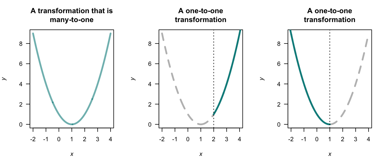
FIGURE 9.1: Three transformations: a non-one-to-one transformation (left panel), and two one-to-one transformations (centre and right panels).

9.2 The change of variable method

The method is relatively straightforward for one-to-one transformations, but considerable care is needed if the transformation is many-to-one (or, many-to-one); examples are given below. The discrete and continuous cases are considered separately.

The functions that are produced should be valid probability functions; check that this is the case.

9.2.1 Discrete random variables

Let \(X\) be a discrete random variable with probability function \(p_X(x)\), and let \(\mathcal{R}_X\) denote the set of discrete points for which \(p_X(x) > 0\). Let \(Y = u(X)\) define a one-to-one transformation that maps \(\mathcal{R}_X\) onto \(\mathcal{R}_Y\), the set of discrete points for which the transformed variable \(Y\) has a non-zero probability. If we solve \(Y = u(X)\) for \(X\) in terms of \(Y\), say \(X = w(Y) = u^{-1}(Y)\), then for each \(y \in \mathcal{R}_Y\), we have \(x = w(y)\in \mathcal{R}_X\).

Example 9.2 (Change of variable method: one discrete rv) Suppose \[ p_X(x) = x/15 \qquad \text{for $x = 1, 2, 3, 4, 5$}. \] To find the probability function of \(Y\) where \(Y = 2X + 1\) (i.e., \(u(x) = 2x + 1\)), first see that \(\mathcal{R}_X = \{1, 2, 3, 4, 5\}\). Hence \(\mathcal{R}_Y = \{3, 5, 7, 9, 11\}\) and the mapping \(y = 2x + 1 = u(x)\) is one-to-one. Also, \(w(y) = u^{-1}(y) = (y - 1)/2\). Hence, \[ \Pr(Y = y) = \Pr(2X + 1 = y) = \Pr\left(X = \frac{y - 1}{2}\right) = \left(\frac{y - 1}{2}\right) \times\frac{1}{15} = \frac{y - 1}{30}. \] So the probability function of \(Y\) is \[ \Pr(Y = y) = (y - 1)/30 \qquad \text{for $y = 3, 5, 7, 9, 11$}. \] (Note: The probabilities in this probability function add to \(1\).)

The above procedure when \(Y = u(X)\) is a one-to-one mapping can be stated generally as \[\begin{align*} \Pr(Y = y) &= \Pr\big(u(X) = y\big)\\ &= \Pr\big(X = u^{-1} (y)\big)\\ &= p_X\big(u^{-1}(y)\big), \quad\text{for $y\in \mathcal{R}_Y$}. \end{align*}\]

Example 9.3 (Transformation (1:1)) Let \(X\) have a binomial distribution with probability function \[ p_X(x) = \begin{cases} \binom{3}{x}0.2^x (0.8)^{3 - x} & \text{for $x = 0, 1, 2, 3$};\\ 0 & \text{otherwise}. \end{cases} \] To find the probability function of \(Y = X^2\), first note that \(Y = X^2\) is not a one-to-one transformation in general, but is one-to-one over the range of \(X\) (i.e., for \(x = 0, 1, 2, 3\)).

The transformation \(y = u(x) = x^2\), \(\mathcal{R}_X = \{x = 0, 1, 2, 3 \}\) maps onto \(\mathcal{R}_Y = \{y = 0, 1, 4, 9\}\). The inverse function is \(x = w(y) = \sqrt{y}\), and hence the probability function of \(Y\) is \[ p_Y(y) = p_X(\sqrt{y}\,) = \begin{cases} \binom{3}{\sqrt{y}}0.2^{\sqrt{y}} (0.8)^{3 - \sqrt{y}} & \text{for $y = 0, 1, 4, 9$};\\ 0 & \text{otherwise}. \end{cases} \]

When the transformation  \(u(\cdot)\) is not 1:1, more care is needed. An example follows.

Example 9.4 (Transformation not 1:1) Suppose \(\Pr(X = x)\) is defined as in Example 9.2, and define \(Y = |X - 3|\). Since \(\mathcal{R}_Y = \{0, 1, 2\}\) the mapping is not one-to-one:

\(\Pr(X = x)\)	\(X\)	\(Y = |X - 3|\)
\(1/15\)	\(1\)	\(2\)
\(2/15\)	\(2\)	\(1\)
\(3/15\)	\(3\)	\(0\)
\(4/15\)	\(4\)	\(1\)
\(5/15\)	\(5\)	\(2\)

So, for example, \(X = 2\) and \(X = 4\) both map to \(Y = 1\). Also, we can see that \(\mathcal{R}_Y = \{ 0, 1, 2\}\).

Then, the probability distribution of \(Y\) is \[\begin{align*} \Pr(Y = 0) &= \Pr(X = 3) = 3/15 = \frac{1}{5};\\ \Pr(Y = 1) &= \Pr(X = 2) + \Pr(X = 4) = \frac{2}{15} + \frac{4}{15} = \frac{2}{5};\\ \Pr(Y = 2) &= \Pr(X = 1) + \Pr(X = 5) = \frac{1}{15} + \frac{5}{15} = \frac{2}{5}. \end{align*}\] The probability function of \(Y\) is \[ p_Y(y) = \begin{cases} 1/5 & \text{for $y = 0$};\\ 2/5 & \text{for $y = 1$};\\ 2/5 & \text{for $y = 2$}. \end{cases} \]

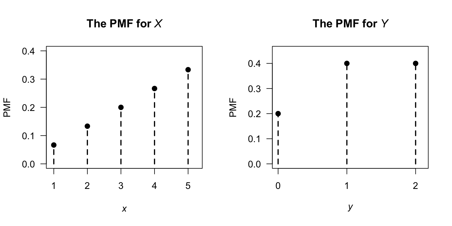
FIGURE 9.2: The PMF for \(X\) and for the transformed variable \(Y\).

9.2.2 Continuous random variables

The change of variable method is similar for continuous random variables, but requires the use of a Jacobian. For a discrete random variable, probability exists at distinct values of the random variable, but probability only exists over intervals for continuous random variables. Suppose the original variable \(X\) has a given probability defined over (say) \(0 < X < 1\); the equivalent probability in the transformed variable \(Y\) may be defined over (say) \(-4 < Y < 4\). The Jacobian is needed to ensure the height of the corresponding density function accommodates this local change in the length of the interval (which may not be linear) over which the equivalent probability is defined.

Theorem 9.1 (Change of variable (continuous rv)) If \(X\) has PDF \(f_X(x)\) for \(x\in \mathcal{R}_X\) and \(u(\cdot)\) is a one-to-one function for \(x\in \mathcal{R}_X\), then the random variable \(Y = u(X)\) has PDF \[ f_Y(y) = f_X(x) \left|\frac{dx}{dy}\right| \] where the right-hand side is expressed as a function of \(y\). The term \(\left|dx/dy\right|\) is called the Jacobian of the transformation.

Proof. Let the inverse function be \(X = w(Y)\) so that \(w(y) = u^{-1}(x)\).

Case 1: \(y = u(x)\) is a strictly increasing function (Fig. 9.3, left panel). If \(a < y < b\) then \(w(a) < x < w(b)\) and \(\Pr(a < Y < b) = \Pr\big(w(a) < X <w(b)\big)\), so \[ {\int^b_a f_Y(y)\,dy =\int^{w(b)}_{w(a)} f_X(x)\,dx =\int^b_a f_X\big( w(y)\big) \frac{dx}{dy}\,\,dy}. \] Therefore, \(\displaystyle {f_Y(y) = f_X\big( w(y) \big)\frac{dx}{dy}}\), where \(w(y) = u^{-1}(x)\).

Case 2: \(y = u(x)\) is a strictly decreasing function of \(x\) (Fig. 9.3, right panel). If \(a < y < b\) then \(w(b) < x < w(a)\) and \(\Pr(a < Y < b) = \Pr\big(w(b) < X < w(a)\big)\), so that \[\begin{align*} \int^b_a f_Y(y)\,dy & = \int^{w(a)}_{w(b)} f_X(x)\,dx\\ & = \int^a_b f_X(x) \frac{dx}{dy}\,\,dy\\ & = - \int ^b_a f_X(x) \frac{dx}{dy}\,dy. \end{align*}\] Therefore \(f_Y(y) = -f_X\left( w(y) \right)\displaystyle{\frac{dx}{dy}}\). Since \(dx/dy\) is negative in the case of a decreasing function, in general \[ f_Y(y) = f_X(x)\left|\frac{dx}{dy} \right|. \]

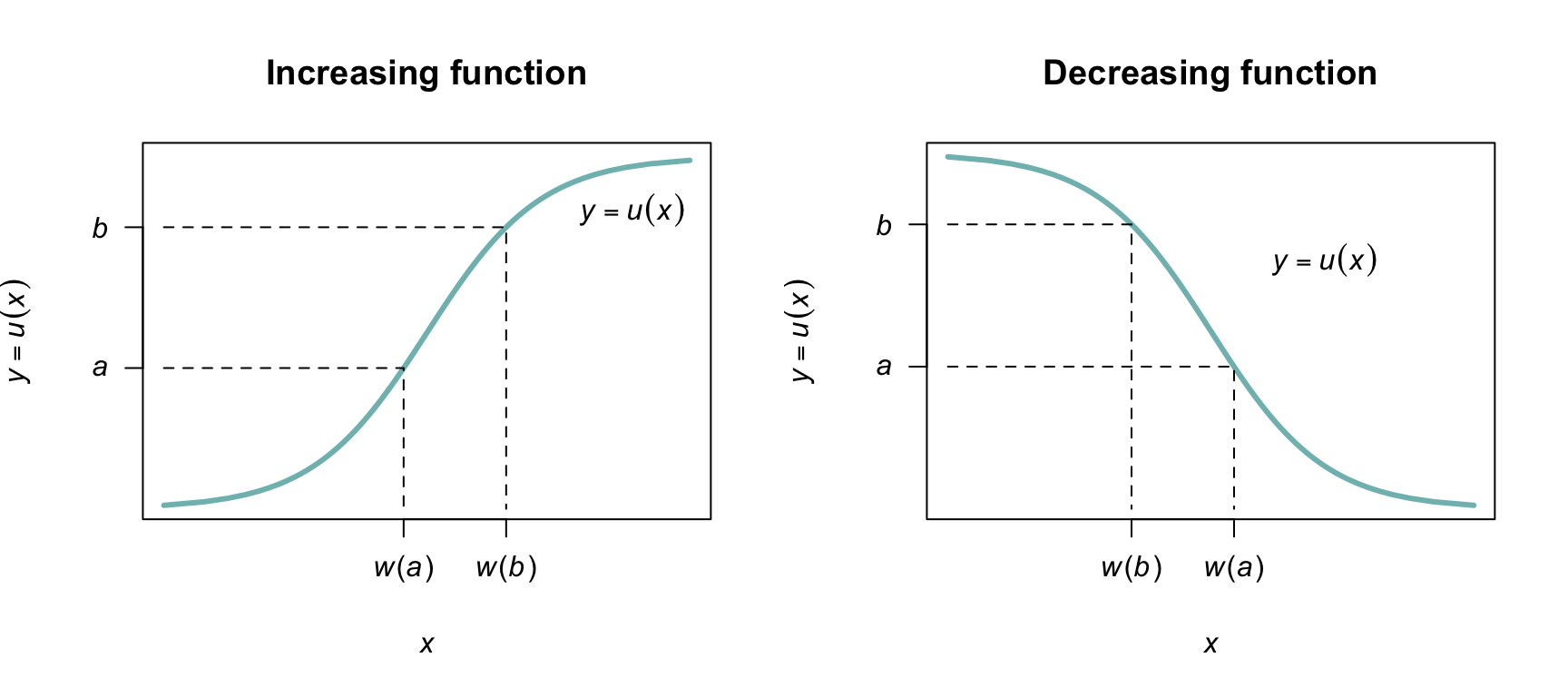
FIGURE 9.3: A strictly increasing one-to-one transformation function (left panel) and strictly decreasing one-to-one function (right panel).

Example 9.5 (Transformation) Let the PDF of \(X\) be given by \[ f_X(x) = 1 \qquad \text{for $0 < x < 1$}. \] Consider the transformation \(Y = u(X) = -2\log X\) (where \(\log\) refers to logarithms to base \(e\), or natural logarithms). The transformation is one-to-one, and the inverse transformation is \[ X = \exp( -Y/2) = u^{-1}(Y) = w(Y). \] The space \(\mathcal{R}_X = \{x \mid 0 < x < 1\}\) is mapped to \(\mathcal{R}_Y = \{y \mid 0 < y < \infty\}\). Then, \[ w'(y) = \frac{d}{dy} \exp(-y/2) = -\frac{1}{2}\exp(-y/2), \] and so the Jacobian of the transformation \(|w'(y)| = \exp(-y/2)/2\). The PDF of \(Y = -2\log X\) is \[\begin{align*} f_Y(y) &= f_X\big(w(y)\big) |w'(y)| \\ &= f_X\big(\exp(-y/2)\big) \exp(-y/2)/2 \\ &= \frac{1}{2}\exp(-y/2)\quad\text{for $y > 0$}. \end{align*}\] That is, \(Y\) has an exponential distribution with \(\beta = 2\): \(Y \sim \text{Exp}(2)\) (Def. 7.7).

Example 9.6 (Square root transformation) Consider the random variable \(X\) with PDF \(f_X(x) = \exp(-x)\) for \(x \geq 0\). To find the PDF of \(Y = \sqrt{X}\), first see that \(y = \sqrt{x}\) is a strictly increasing function for \(x \geq 0\) (Fig. 9.4).

The inverse relation is \(X = Y^2\), and \(dx/dy = |2y| = 2y\) for \(x \ge 0\). The PDF of \(Y\) is \[ f_Y(y) = f_X(x)\left|\frac{dx}{dy}\right| = 2y \exp(-y^2)\quad \text{for $y\geq0$}. \]

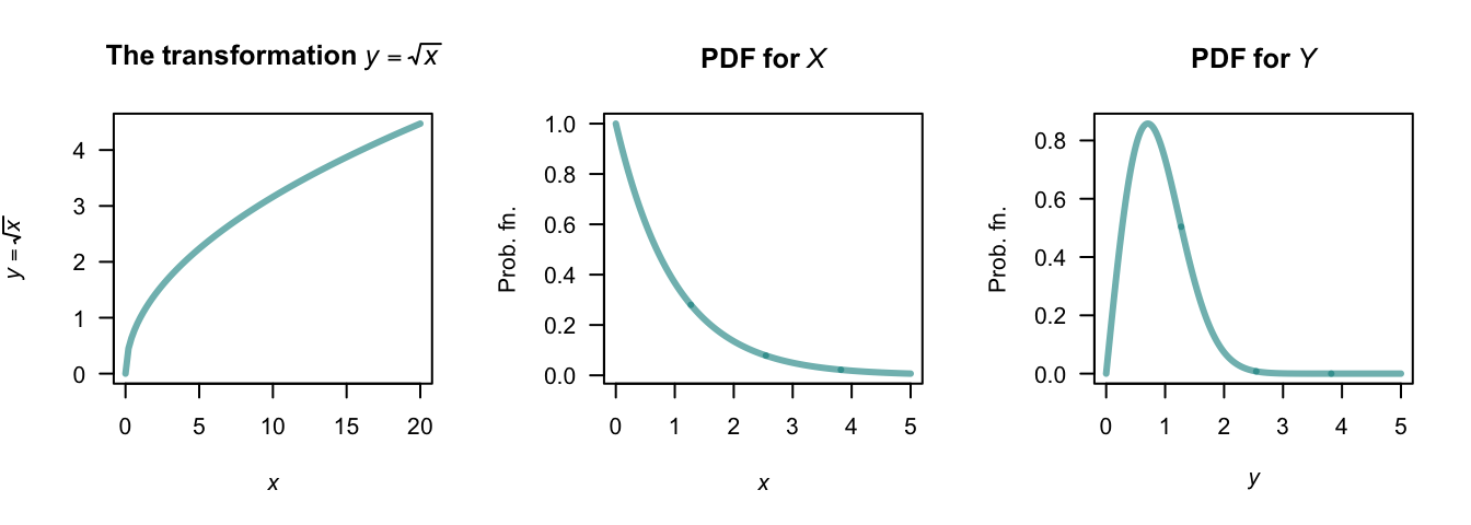
FIGURE 9.4: The square-root transformation (left panel); the PDF of \(X\) (centre panel) and the PDF of \(Y\) (right panel).

Example 9.7 (Tan transformation) Let random variable \(X\) be uniformly distributed on \((-\pi/2, \pi/2)\) Fig. 9.5 (centre panel). Suppose we seek the distribution of \(Y = \tan X\) (Fig. 9.5, left panel).

For the mapping \(Y = \tan X\), we see that \(\mathcal{R}_Y = \{ y\mid -\infty <y<\infty\}\). The mapping is one-to-one, and so \(X = \tan^{-1}Y\), and \(dx/dy = 1/(1 + y^2)\). Hence \[ f_Y(y) = f_X(x)\left|\frac{dx}{dy}\right| = \frac{1}{\pi(1 + y^2)}. \] The distribution is shown in Fig. 9.5 (right panel). This is the Cauchy distribution.

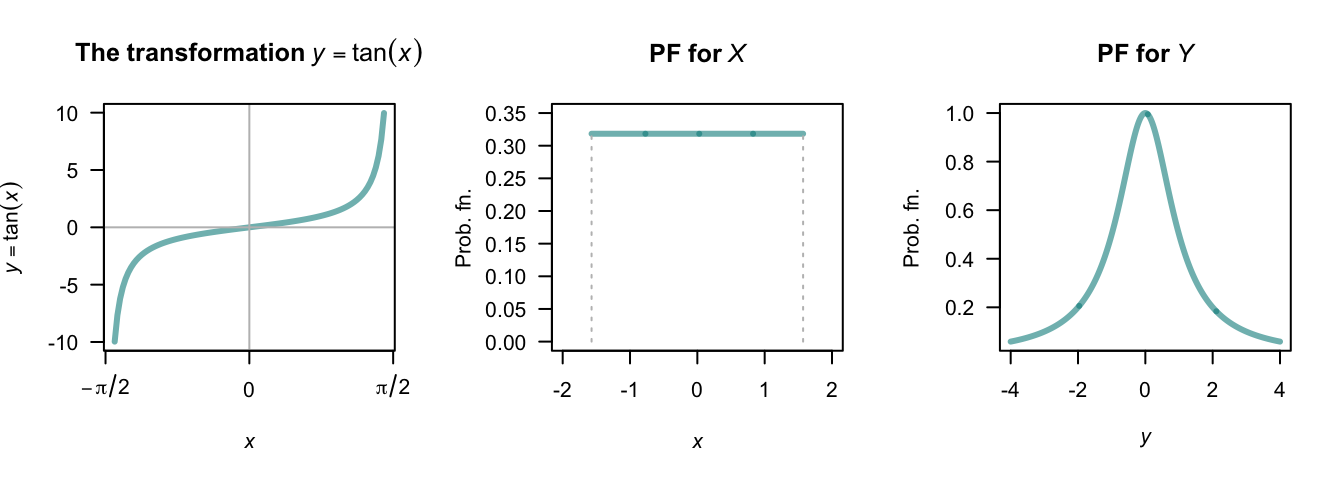
FIGURE 9.5: The tan transformation (left panel); the PDF of \(X\) (centre panel) and the PDF of \(Y\) (right panel).

In cases where the function \(u(\cdot)\) is not a one-to-one transformation over \(\mathcal{R}_X\), usually \(\mathcal{R}_X\) can be split into smaller sets where the transformation is one-to-one in each. We give an example next.

Example 9.8 (Transformation (not 1:1)) Given a random variable \(Z\) which follows a \(N(0, 1)\) distribution, suppose we seek the probability distribution of \(Y = \frac{1}{2} Z^2\). Then: \[ f_Z(z) = \frac{1}{\sqrt{2\pi}}\,\exp\left( -\frac{1}{2} z^2\right)\quad\text{for $-\infty < z < \infty$}. \] The inverse relation, \(Z = u^{-1}(Y)\) is \(Z = \pm \sqrt{2Y}\), which is not strictly increasing or decreasing on \(\mathcal{R}_Z = (-\infty, \infty )\), so Theorem 9.1 cannot be applied directly.

However, the support \(\mathcal{R}_Z\) can be partitioned into two regions where the transformation is one-to-one: \(Z \le 0\) (Region A) and \(Z > 0\) (Region B), where the equality could be in either partition. This is shown in Fig. 9.6. Values of \(a < y < b\) correspond to two regions in \(\mathcal{R}_Z\) (one in each partition): \(-\sqrt{2b} < z < -\sqrt{2a}\) in Region A, and \(\sqrt{2a} < z < \sqrt{2b}\) in Region B. Thus, \[\begin{align*} \Pr(a < Y <b) = &\Pr(-\sqrt{2b} < Z < -\sqrt{2a}\,) + {}\\ &\Pr( \sqrt{2a} < Z < \sqrt{2b}\,). \end{align*}\] The two terms on the right are equal because the distribution of \(Z\) is symmetrical about \(z = 0\), and so \(\Pr(a < Y < b) = 2\Pr(\sqrt{2a} < Z < \sqrt{2b}\,)\). So we can write \[\begin{align*} f_Y(y) &= 2f_Z(z)\left| \frac{dz}{dy}\right|\\ &= 2\frac{1}{\sqrt{2\pi}}\exp(-y)\frac{1}{\sqrt{2y}}; \end{align*}\] that is, \[ f_Y(y) = \exp(-y) y^{-\frac{1}{2}} / \sqrt{\pi}\quad\text{for $0 < y < \infty$}. \] This PDF is a gamma distribution (Sect. 7.5) with parameters \(\alpha = 1/2\) and \(\beta = 1\).

It follows that if \(X\sim N(\mu,\sigma^2)\), then the PDF of \(Y = \frac{1}{2} (X - \mu )^2 / \sigma^2\) is \(\text{Gamma}(\alpha = 1/2,\beta = 1)\) since then \((X - \mu)/\sigma\) is distributed as \(N(0, 1)\).

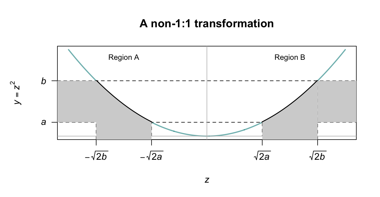
FIGURE 9.6: A transformation that is not 1:1. The transformation is one-to-one in the two regions, Region A and Region B.

Note that the probability can only be doubled as in Example 9.8 if both \(Y = u(Z)\) and the PDF of \(Z\) are symmetrical about the same point.

9.2.3 Summary

The change of variable method requires find the pre-image, then accounting for the how transformation redistributes probability (through counting in the discrete case; through the Jacobian in the continuous case); see Table 9.1.

TABLE 9.1: Summarising the change of variable method.

Setting	Discrete	Continuous
Univariate	Sum \(p_X(x)\) over every \(x\) that transforms into \(y\)	Substitute inverse; multiply by \(|\det J|\)
Bivariate	Sum \(p_{X_1, X_2}(x_1, x_2)\) over every \((x_1, x_2)\) that transforms into \((y_1, y_2)\)	Substitute inverses; multiply by \(|\det J|\)

9.3 The distribution function method

The distribution function method is the most broadly applicable technique for finding the distribution of a transformed random variable. The strategy is to:

1. Write \(F_Y(y) = \Pr(Y \leq y) = \Pr(g(X) \leq y)\).
2. Re-express the event \(\{g(X) \leq y\}\) as an equivalent event in terms of \(X\).
3. Evaluate using the known distribution of \(X\).
4. Differentiate (continuous case) or take differences (discrete case) to obtain the PDF: \(f_Y(y) = F_Y'(y)\).

The distribution function method operates with probabilities rather than densities, so it works with non-monotone transformations, awkward supports, and many-to-one mappings without requiring the special conditions needed with the change of variables method (i.e., one-to-one transformations; differentiable transformations).

The functions that are produced should be valid probability functions; check that this is the case.

9.3.1 Continuous random variables

The general procedure above is best demonstrated using an example.

Example 9.9 (Distribution function method) Consider the random variable \(X\) with PDF \[ f_X(x) = x/4 \qquad \text{for $1 < x < 3$}. \] To find the PDF of the random variable \(Y\) where \(Y = X^2\), first see that \(1 < y < 9\) and the transformation is monotonic over this region. The distribution function for \(Y\) is \[\begin{align*} F_Y(y) &= \Pr(Y\le y) \qquad\text{(by definition)}\\ &= \Pr(X^2 \le y) \qquad\text{(since $Y = X^2$)}\\ &= \Pr(X\le \sqrt{y}\,). \end{align*}\] This last step is not trivial, but is critical. Sometimes, more care is needed (see Example 9.10). In this case, there is a one-to-one relationship between \(X\) and \(Y\) over the region of which \(X\) is defined (i.e., has a positive probability); see Fig. 9.7.

Then continue as follows: \[\begin{align*} F_Y(y) =\Pr( X\le \sqrt{y}\,) &= F_X\big(\sqrt{y}\,\big) \qquad\text{(definition of $F_X(x)$)} \\ &= \int_1^{\sqrt{y}} (x/4) \,dx = (y - 1)/8 \end{align*}\] for \(1 < y < 9\). This is the distribution function of \(Y\); the PDF is \[ f_Y(y) = \frac{d}{dy} (y - 1)/8 = 1/8 \qquad \text{for $1 < y < 9$}. \] Note the range for which \(Y\) is defined; since \(1 < x < 3\), then \(1 < y < 9\).

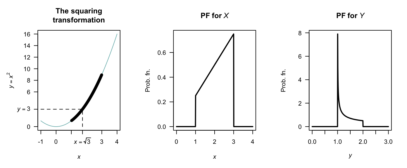
FIGURE 9.7: The transformation \(Y = X^2\) when \(X\) is defined from \(1\) to \(3\). The thicker line corresponds to the region where the transformation applies. Note that if \(Y < y\), then \(2 - \sqrt{y - 1} < X < 2 + \sqrt{y - 1}\).

Example 9.10 (Transformation) Consider the same random variable \(X\) as in the previous example, but the transformation \(Y = (X - 2)^2 + 1\) (Fig. 9.8).

In this case, the transformation is not a one-to-one transform. Proceed as before to find the distribution function of \(Y\): \[\begin{align*} F_Y(y) &= \Pr(Y\le y) \qquad\text{(by definition)}\\ &= \Pr\big( (X - 2)^2 + 1 \le y\big) \end{align*}\] since \(Y = (X - 2)^2 + 1\). From Fig. 9.8, whenever \((X - 2)^2 + 1 < y\) for some value \(y\), then \(X\) must be in the range \(2 - \sqrt{y - 1}\) to \(2 + \sqrt{y - 1}\). So: \[\begin{align*} F_Y(y) &= \Pr\big( (X - 2)^2 + 1 \le y\big) \\ &= \Pr\left( 2 - \sqrt{y - 1} < X < 2 + \sqrt{y - 1} \right)\\ &= \int_{2-\sqrt{y - 1}}^{2 + \sqrt{y - 1}} x/4\,dx \\ &= \sqrt{y - 1}. \end{align*}\] Again, this is the distribution function; so differentiating to find the PDF gives \[ f_Y(y) = \frac{1}{2\sqrt{y - 1}} \qquad \text{for $1 < y < 2$}. \]

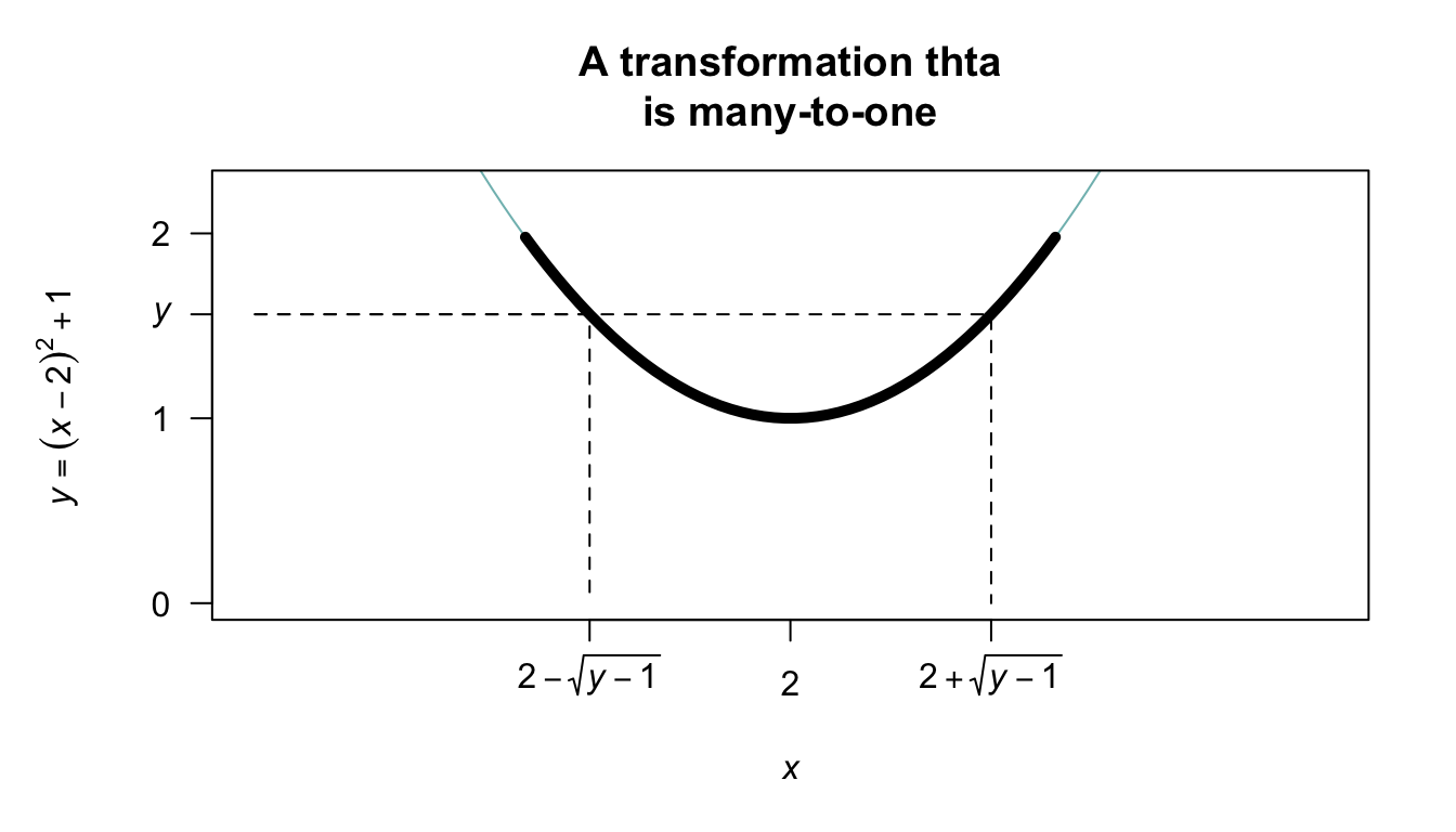
FIGURE 9.8: The transformation \(Y = (X - 2)^2 + 1\) when \(X\) is defined from \(1\) to \(3\). The thicker line corresponds to the region where the transformation applies. Note that if \(Y < y\), then \(2 - \sqrt{y - 1} < X < 2 + \sqrt{y - 1}\).

Example 9.11 (Transformation) Example 9.8 is repeated here using the distribution function method. Given \(Z\) is distributed \(N(0, 1)\) we seek the probability distribution of \(Y = \frac{1}{2} Z^2\). First, \[ f_Z(z) = (2\pi )^{-\frac 12}\,\exp(-z^2/2)\quad\text{for $z\in (-\infty ,\,\infty )$}. \] Let \(Y\) have PDF \(f_Y(y)\) and df \(F_Y(y)\). Then \[\begin{align*} F_Y(y) = \Pr(Y\leq y) &= \Pr\left(\frac{1}{2}Z^2\leq y\right)\\ &= \Pr(Z^2\leq 2y)\\ & = \Pr(-\sqrt{2y}\leq Z\leq \sqrt{2y}\,)\\ & = F_Z(\sqrt{2y}\,) - F_Z(-\sqrt{2y}\,) \end{align*}\] where \(F_Z\) is the distribution function of \(Z\). Hence \[\begin{align*} f_Y(y) = F_Y'(y) &= F_Z'(\sqrt{2y}\,)-F_Z'(-\sqrt{2y}\,)\\ &= \frac{\sqrt{2}}{2\sqrt{y}}f_Z(\sqrt{2y}\,) - \frac{\sqrt{2}}{-2\sqrt{y}}f_Z(-\sqrt{2y}\,)\\[2mm] &= \frac{1}{\sqrt{2y}}[f_Z(\sqrt{2y}\,) + f_Z(-\sqrt{2y}\,)]\\ &= \frac{1}{\sqrt{2y}} \left[ \frac{1}{\sqrt{2\pi}}\,\exp(-y) + \frac{1}{\sqrt{2\pi}}\,\exp(-y)\right]\\ &= \frac{\exp(-y)\,y^{-\frac{1}{2}}}{\sqrt{\pi}} \end{align*}\] as before.

Example 9.12 (Distribution function method, with two parts) Consider the random variable \(X\) with the probability density function (Fig. 9.9, left panel) \[ f_X(x) = \begin{cases} 1/2 & \text{for $0 < x < 1$};\\ (3 - x)/4 & \text{for $1 < x < 3$.} \end{cases} \] Then, consider the distribution of \(Y = X^2\); then, \(0 < y < 9\). More specifically, \(\{ x \mid 0 < x < 1\}\) maps to \(\{y \mid 0 < y < 1\}\) and \(\{ x \mid 1 < x < 3\}\) maps to \(\{y \mid 1 < y < 9\}\).

To use the distribution function method, the distribution function of \(X\) is needed: \[ F_X(x) = \begin{cases} 0 & \text{for $x < 0$}\\ x/2 & \text{for $0 < x < 1$};\\ -(x^2 - 6x + 1)/8 & \text{for $1 < x < 3$}\\ 1 & f\text{for $x \ge 3$}. \end{cases} \] Then proceed: \[\begin{align*} F_Y(y) &= \Pr(Y \le y)\\ &= \Pr(X^2 \le y)\\ &= \Pr(X \le \sqrt{Y})\\ &= F_X(\sqrt{y}\,)\\ &= \begin{cases} \sqrt{y}/2 & \text{for $0 < y < 1$}\\ -(y - 6\sqrt{y} + 1)/8 & \text{for $1 < y < 9$}. \end{cases} \end{align*}\] To recover the PDF of \(Y\) (Fig. 9.9, right panel), differentiate to obtain \[ f_Y(y) = \begin{cases} \displaystyle \frac{1}{4\sqrt{y}} & \text{for $0 < y < 1$}\\[6pt] \displaystyle \frac{3}{8\sqrt{y}} - \frac{1}{8} & \text{for $1 < y < 9$}. \end{cases} \]

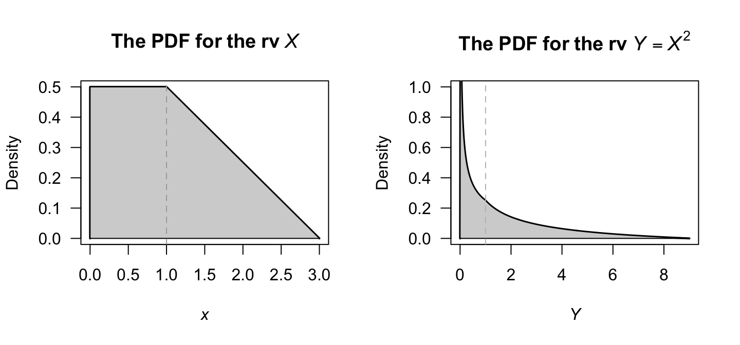
FIGURE 9.9: The probability density functions of \(X\) (left) and \(Y = X^2\) (right).

Care is needed to ensure the steps are followed logically. Diagrams like Fig. 9.7 and 9.8 are encouraged.

Example 9.13 (Proof of Theorem 5.1) Theorem 5.1 gave an important theorem involving the expectation of function of a random variable. Here, we prove this theorem for the discrete and continuous cases.

For the discrete case , we need to show that \(\sum_{\mathcal{R}_Y} y\cdot \Pr(u(X) = y) = \sum_x u(x)\, \Pr(X = x)\) for \(y \in \mathcal{R}_Y\), for some transformation \(Y = u(X)\).

By definition, \(\operatorname{E}[Y] = \sum_{\mathcal{R}_Y} y\cdot \Pr(Y = y)\). Recall that the event \(\{Y = y\}\) is actually the set of all \(x\) such that \(u(x) = y\), so substituting gives \(\Pr(Y = y) = \sum_{x: u(x) = y} \Pr(X = x)\). Substituting this into the expectation: \[ \operatorname{E}[u(X)] = \sum_{\mathcal{R}_Y} y \left( \sum_{x: u(x) = y} \Pr(X = x) \right). \] Since \(y = u(x)\) for all \(x\) in the inner sum, it can be moved inside the inner summation: \[\begin{align*} \operatorname{E}[u(X)] &= \sum_{\mathcal{R}_Y} \sum_{x: u(x) = y} y\cdot \Pr(X = x)\\ &= \sum_{\mathcal{R}_Y} \sum_{x: u(x) = y} u(x)\cdot \Pr(X = x). \end{align*}\] The double sum partitions the range of \(X\), so every \(x\) appears exactly once. In other words, \(\operatorname{E}[u(X)] = \sum_x u(x) \Pr(X = x)\).

For the continuous case, we need to show that \(\int_{-\infty}^\infty y\cdot f_Y(y)\, dy = \int_{-\infty}^\infty u(x)\, f_X(x)\, dx\).

Assume \(u(x)\) is a strictly increasing, differentiable function (this makes the proof simpler, but the result applies more generally). Let \(Y = u(X)\). Find the PDF of \(Y\) using the transformation method: \[ f_Y(y) = f_X(x) \left| \frac{dx}{dy} \right| \quad \text{where } x = u^{-1}(y). \] Then, using the definition of \(\operatorname{E}[Y]\): \[ \operatorname{E}[Y] = \int_{-\infty}^{\infty} y\cdot f_Y(y) \, dy. \] Substitute \(y = u(x)\) and \(f_Y(y)\, dy = f_X(x)\, dx\): \[\begin{align*} \operatorname{E}[Y] &= \int_{-\infty}^{\infty} u(x) \cdot f_X(x) |u'(x)| \cdot \frac{1}{|u'(x)|} \, dx\\ &= \int_{-\infty}^{\infty} u(x)\,f_X(x)\,dx \end{align*}\]

Example 9.14 (Distribution of squared normal rv) Let \(X \sim N(0, 1)\) and \(Y = X^2\). Since \(u(x) = x^2\) is not monotone on \(\mathbb{R}\), the change of variable method requires partitioning; the distribution function method is simpler.

First, see that the support for \(X\) is over \(\mathbb{R}\), but the support for \(Y = X^2\) must be over the non-negative reals. Furthermore, since individual points have zero probability for continuous random variables, \(X = 0\) is not technically possible, so the support is best given as \((0, \infty)\) or \([0, \infty)\) (see Fig. 9.10).

So, for \(y > 0\): \[ F_Y(y) = \Pr(X^2 \leq y) = \Pr(-\sqrt{y} \leq X \leq \sqrt{y}\,) = F_X(\sqrt{y}\,) - F_X(-\sqrt{y}\,) = 2F_X(\sqrt{y}\,) - 1. \]

Differentiating: \[ f_Y(y) = 2 f_X(\sqrt{y}\,) \cdot \frac{1}{2\sqrt{y}} = \frac{1}{\sqrt{y}} \cdot \frac{1}{\sqrt{2\pi}} \exp(-y/2) = \frac{y^{1/2 - 1} \exp(-y/2)}{2^{1/2}\,\Gamma(1/2)}, \quad y > 0. \] Notice that \(Y > 0\); if \(Y = 0\) the PMF is undefined. The final expressions identifies this as the \(\chi^2(1)\) distribution (i.e., \(\text{Gamma}(1/2,\, 1/2)\)).

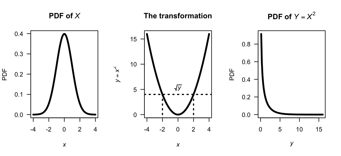
FIGURE 9.10: A normal distribution (left panel), the transformation (centre panel), and the resulting chi-squared distribution (right panel).

9.3.2 Discrete univariate case

Let \(X\) be a discrete random variable with PMF \(p_X(x)\) and CDF \(F_X(x) = \Pr(X \leq x)\). For \(Y = u(X)\), the CDF of \(Y\) is \[ F_Y(y) = \Pr(Y \leq y) = \Pr(u(X) \leq y) = \sum_{\{x:\, u(x) \leq y\}} p_X(x). \] The PMF of \(Y\) is then recovered as \[ p_Y(y) = F_Y(y) - F_Y(y^-) \] where \(y^-\) denotes the largest value in the support of \(Y\) that is strictly less than \(y\). When \(Y\) takes consecutive integer values (such as \(\{0, 1, 2, \dots\}\) or \(\{1, 2, 3, \dots\}\)), this simplifies to \(F_Y(y) - F_Y(y - 1)\).

In the discrete case, the CDF method and the change of variables method are closely related; the difference is mainly one of presentation. The distribution function is especially natural when \(u(\cdot)\) is monotone non-decreasing, since the event \(\{u(X) \leq y\}\) maps cleanly to \(\{X \leq u^{-1}(y)\}\).

Example 9.15 (Shifting the geometric distribution) Let \(X \sim \text{Geometric}(p)\), so that \(X\) represents the number of failures until the first success, with support \(\{0, 1, 2, \ldots\}\) (as in Sect. 6.5). Then, \[ \Pr(X \leq x) = 1 - (1-p)^{\lfloor x\rfloor + 1}, \quad x = 0, 1, 2, \ldots \] Define \(Y = X + 1\), so that \(Y\) is the number of trials up to and including the first success, with support \(\{1, 2, 3, \ldots\}\). For \(y \in \{1, 2, 3, \ldots\}\): \[\begin{align*} F_Y(y) = \Pr(Y \leq y) &= \Pr(X + 1 \leq y)\\ &= \Pr(X \leq y - 1)\\ &= 1 - (1 - p)^{(y - 1) + 1}\\ &= 1 - (1 - p)^{y}, \end{align*}\] using the DF for \(X\) above. The PMF is the difference between the DF at the values of \(Y\) with positive probabilities (see Sect. 4.4.5): \[ p_Y(y) = F_Y(y) - F_Y(y - 1) = (1 - p)^{y - 1} p, \quad y = 1, 2, 3, \ldots \] This is the \(\text{Geometric}(p)\) distribution with a different parameterisation. A simple shift of support corresponds to a reparameterisation within the geometric family of distributions.

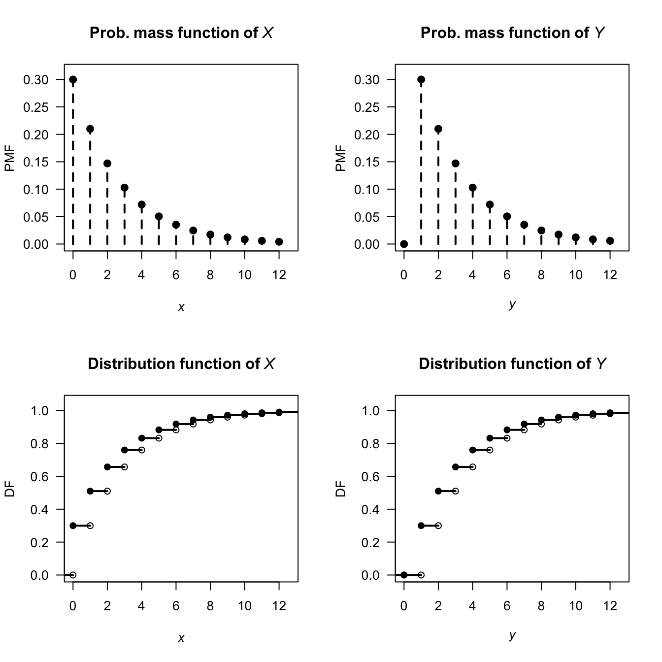
FIGURE 9.11: The PMF and DF of \(X\) following a geometric distribution (left panels), and the PMF and DF of the transformation \(Y = X + 1\).

9.3.3 Summary

The distribution function method is preferred over the change of variables method when

1. the transformation is many-to-one (e.g. maximum, minimum, absolute value);
2. the result is not a standard named distribution; or
3. only a marginal distribution is needed from a multivariate problem.

The approach is summarised in Table 9.2.

TABLE 9.2: Summarising the distribution function method.

Setting	Strategy	PDF recovery
Discrete univariate	\(F_Y(y) = \sum_{\{x:\,g(x)\leq y\}} p_X(x)\); pmf = \(\Delta F_Y\)	Difference the CDF
Continuous univariate	\(F_Y(y) = \Pr(g(X)\leq y)\); invert inequality; use \(F_X\)	Differentiate the CDF
Discrete bivariate	\(F_Y(y) = \iint_{\{g\leq y\}} f_{X_1, X_2}\); characterise region	Differentiate the CDF
Continuous bivariate	\(F_Y(y) = \sum\sum_{\{g\leq y\}} p_{X_1, X_2}\); pmf = \(\Delta F_Y\)	Difference the CDF

9.4 The moment generating function method

The moment generating function (MGF) method is useful for finding the distribution of a linear combination of \(n\) independent random variables. The method essentially involves the computation of the MGF of the transformed variable \(Y = u(X_1, X_2, \dots, X_n)\) when the joint distribution of independent \(X_1, X_2, \dots, X_n\) is given.

The MGF method relies on this observation: since the MGF of a random variable (if it exists) completely specifies the distribution of the random variable, then if two random variables have the same MGF they must have identical distributions. Below, the transformation \(Y = X_1 + X_2 + \cdots X_n\) is demonstrated, but the same principles can be applied for other linear combinations also.

Consider \(n\) independent random variables \(X_1, X_2, \dots, X_n\) with MGFs \(M_{X_1}(t)\), \(M_{X_2}(t)\), \(\dots\), \(M_{X_n}(t)\), and consider the transformation \(Y = X_1 + X_2 + \cdots X_n\). Since the \(X_i\) are independent, \(f_{X_1,X_2\dots X_n}(x_1, x_2, \dots, x_n) = f_{X_1}(x_1).f_{X_2}(x_2)\dots f_{X_n}(x_n)\). So, by definition of the MGF, \[\begin{align*} M_Y(t) &= \operatorname{E}[\exp(tY)] \\ &= \operatorname{E}[\exp(t(X_1 + X_2 + \cdots X_n))] \\ &= \int\!\!\!\int\!\!\!\cdots\!\!\!\int \exp[t(x_1 + x_2 + \cdots x_n)] f(x_1, x_2, \dots x_n)\,dx_n\dots dx_2\, dx_1 \\ &= \int\!\!\!\int\!\!\!\cdots\!\!\!\int \exp(tx_1) f(x_1) \exp(t{x_2}) f(x_2)\dots \exp(t{x_n})f(x_n) \,dx_n\dots dx_2\, dx_1 \\ &= \int \exp(t x_1) f(x_1)\,dx_1 \int \exp(t{x_2}) f(x_2)\,dx_2 \dots \int \exp(t{x_n})f(x_n)\,dx_n \\ &= M_{X_1}(t) M_{X_2}(t)\dots M_{X_n}(t) \\ &= \prod_{i = 1}^n M_{X_i}(t). \end{align*}\] (\(\prod\) is the symbol for a product of terms, in the same way that \(\sum\) is the symbol for a summation of terms.) The above result also holds for discrete variables, where summations replace integrations.

This result follows: if \(X_1, X_2, \dots, X_n\) are independent random variables and \(Y = X_1 + X_2 + \dots + X_n\), then the MGF of \(Y\) is \[ M_Y(t) = \prod_{i = 1}^n M_{X_i}(t) \] where \(M_{X_i}(t)\) is the MGF of \(X_i\) at \(t\) for \(i = 1, 2, \dots, n\).

Example 9.16 (MGF method for transformations) Suppose that \(X_i \sim \text{Poisson}(\lambda_i)\) for \(i = 1, 2, \dots, n\), and we wish to find the distribution of \(Y = X_1 + X_2 + \dots + X_n\).

Since \(X_i\) has a Poisson distribution with parameter \(\lambda_i\) for \(i, 2, \dots n\), the MGF of \(X_i\) is \[ M_{X_i}(t) = \exp[ \lambda_i(\exp t - 1)]. \] The MGF of \(Y = X_1 + X_2 + \cdots X_n\) is \[\begin{align*} M_Y(t) &= \prod_{i = 1}^n \exp[ \lambda_i(\exp t - 1)] \\ &= \exp[ \lambda_1(\exp t - 1)] \exp[ \lambda_2(\exp t - 1)] \dots \exp[ \lambda_n(\exp t - 1)] \\ &= \exp\left[ (\exp t - 1)\sum_{i = 1}^n \lambda_i\right]. \end{align*}\] Using \(\Lambda = \sum_{i = 1}^n \lambda_i\), the MGF of \(Y\) is \[ M_Y(t) = \exp\left[ (\exp t - 1)\Lambda \right], \] which is the MGF of a Poisson distribution with mean \(\Lambda = \sum_{i = 1}^n \lambda_i\). This means that the sum of \(n\) independent Poisson distribution is also a Poisson distribution, whose mean is the sum of the individual Poisson means.

9.5 Choosing a method

The change of variables method is used when the transformation is smooth and monotone (or piecewise monotone), and the full (joint) distribution is required. In the discrete case, the change of variable method is effectively careful bookkeeping rather than a distinct technique. The change of variable method is best avoided when the Jacobian computation is intractable or difficult, or when the full PDF is not needed and only moments are of interest.

The distribution function method is the most general method: it works for any transformation, discrete or continuous. It is also intuitive: compute \(\Pr(Y \le y)\) and differentiate or find differences. The distribution function method, however, can become algebraically tedious, and can become complicated with multivariate or multi-step transformations.

The MGF method is only useful in very specific situations, but in these situations it excels. It is most applicable for sums of random variables; for example, proving that a sum (or linear combination) of independent random variables follows a particular named distribution, since the MGFs are multiplied, and the resulting MGF matched to MGFs of known distributions. The MGF method cnbe used, for example, to show that the sum of independent normal distributions is a normal distributions, that the sum of independent Poisson distributions sum to Poisson distributions, and so on. However, the MGF may not exist, and the method reveals nothing about the joint distribution of a transformed vector; it is useless when the transformation is not a sum or linear combination.

9.6 Exercises

Selected answers appear in Sect. F.8.

Exercise 9.1 Suppose the PDF of \(X\) is given by \[ f_X(x) = x/2 \quad \text{$0 < x < 2$}. \]

1. Find the PDF of \(Y = X^3\) using the change of variable method.
2. Find the PDF of \(Y = X^3\) using the distribution function method.
3. Plot the PDF of \(X\) and \(Y\).

Exercise 9.2 Suppose the PDF of \(X\) is given by \[ f_X(x) = \frac{4}{3} - x^2 \quad \text{$0 < x < 1$}.\\ \]

1. Find the PDF of \(Y = \sqrt{X}\) using the change of variable method.
2. Find the PDF of \(Y = \sqrt{X}\) using the distribution function method.
3. Plot the PDF of \(X\) and \(Y\).

Exercise 9.3 Consider \(n\) random variables \(X_i\) such that \(X_i \sim \text{Gamma}(\alpha_i, \beta)\). Determine the distribution of \(Y = \sum_{i = 1}^n X_i\) using MGFs.

Exercise 9.4 The random variable \(X\) has PDF \[ f_X(x) = \frac{1}{\pi(1 + x^2)} \] for \(-\infty < x < \infty\). Find the PDF of \(Y\) where \(Y = X^2\).

Exercise 9.5 A random variable \(X\) has distribution function \[ F_X(x) = \begin{cases} 0 & \text{for $x \le -0.5$};\\ (2x + 1)/2 & \text{for $-0.5 < x < 0.5$};\\ 1 & \text{for $x \ge 0.5$}. \end{cases} \]

1. Find, and plot, the PDF of \(X\).
2. Find the distribution function, \(F_Y(y)\), of the random variable \(Y = 4 - X^2\).
3. Hence find, and plot, the PDF of \(Y\), \(f_Y(y)\).

Exercise 9.6 Suppose the random variable \(Z\) has the PDF \[ f_Z(z) = \frac{1}{4} \qquad \text{for $-1 < z < 3$}. \]

1. Find the probability density function of \(Y\), where \(Y = Z^2\), using the distribution function method.
2. Confirm that your final PDF of \(Y\) is a valid PDF.
3. Produce a well-labelled plot of the PDF of \(Y\). Ensure all important features and points are clearly labelled.

Exercise 9.7 Suppose the random variable \(X\) has the PDF \[ f_Z(z) = \frac{1}{3} \qquad \text{for $-1 < z < 2$}. \]

1. Find the probability density function of \(Y\), where \(Y = |Z|\), using the distribution function method.
2. Confirm that your final PDF of \(Y\) is a valid PDF.
3. Produce a well-labelled plot of the PDF of \(Y\). Ensure all important features and points are clearly labelled.

Exercise 9.8 Suppose a projectile is fired at an angle \(\theta\) from the horizontal with velocity \(v\). The horizontal distance that the projectile travels \(D\) is \[ D = \frac{v^2}{g} \sin 2\theta, \] where \(g\) is the acceleration due to gravity (\(g\approx 9.8\) m.s^\(-2\)).

1. If \(\theta\) is uniformly distributed over the range \((0, \pi/4)\), find the probability density function of \(D\).
2. Sketch the PDF of \(D\) over a suitable range for \(v = 12\) and using \(g\approx 9.8\)m.s^\(-2\).

Exercise 9.9 In a simple electric circuit, the relationship between voltage \(V\) (in volts), current \(I\) (in amperes) and resistance \(R\) (in ohms) is \[ V = I \cdot R. \] Suppose the supply voltage is constant at \(V = 240\,\text{V}\). The resistance varies between components and is modelled using a log-normal distribution \[ R \sim\text{Log-normal}(\mu = \log 10, \sigma^2 = 0.1), \] so that the median resistance is \(10\) ohms.

1. Find the distribution of \(I\).
2. Sketch the probability distribution of \(I\).
3. Find \(\Pr(I > 30)\).
4. Find \(\operatorname{E}[I]\).
5. Find \(\operatorname{var}[I]\).
6. Compare median of \(I\) with \(240/\operatorname{E}[R]\), and comment.

Exercise 9.10 Most computers have facilities to generate continuous uniform (pseudo-)random numbers between zero and one, say \(X\). When needed, exponential random numbers are obtained from \(X\) using the transformation \(Y = -\alpha\ln X\).

1. Show that \(Y\) has an exponential distribution and determine its parameters.
2. Deduce the mean and variance of \(Y\).

Exercise 9.11 Consider a random variable \(W\) for which \(\Pr(W = 2) = 1/6\), \(\Pr(W = -2) = 1/3\) and \(\Pr(W = 0) = 1/2\).

1. Plot the probability function of \(W\).
2. Find the mean and variance of \(W\).
3. Determine the distribution of \(V = W^2\).
4. Find the distribution function of \(W\).

Exercise 9.12 In a study to model the load on bridges (Lu et al. 2019), the researchers modelled the Gross Vehicle Weight (GVM, in kilonewtons) weight of smaller trucks \(S\) using \(S\sim N(390, 740\), and the weight of bigger trucks \(B\) using \(L\sim N(865, 142)\). The total load distribution \(L\) was then modelled as \(L = 0.24S + 0.76B\), reflecting the expected proportion if smaller and bigger trucks using the bridge.

1. Plot the distribution of \(L\).
2. Compute the mean and standard deviation of \(L\).

Exercise 9.13 The time taken to run a distance \(D\) (in metres) by a professional athlete, say \(T\) (in seconds), varies with the distribution shown in Fig. 9.12 (left panel). The average velocity of the runner, say \(V\), is related to the time by \(V = D/T\).

1. Determine the probability density function for the runner’s velocity.
2. Suppose \(D = 100\), \(\mu = 12\) and \(\Delta = 0.25\). Plot the probability density function for \(V\).

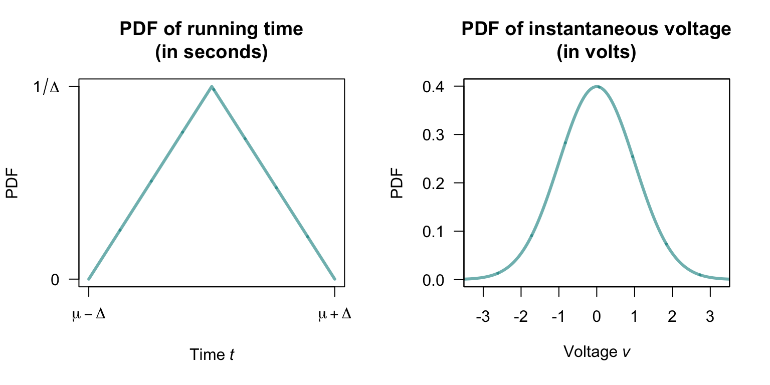
FIGURE 9.12: The probability density function for the random variable \(T\), the time for the run.

Exercise 9.14 Suppose the instantaneous voltage \(V\) (in volts) in a circuit varies over time such that \[ f_V(v) = \frac{1}{\sqrt{2\pi\sigma^2}}\exp\left\{ -\frac{x^2}{2\sigma^2}\right\}. \] as shown in Fig. 9.12 (right panel).

1. Determine the probability density function of the instantaneous power in the circuit \(P\), where \(P = V^2/R\) for some circuit resistance \(R\) (in ohms).
2. Suppose \(\sigma = 1\), and \(R = 10\). Plot the probability density function for \(P\).

Exercise 9.15 Suppose the random variable \(X\) has a normal distribution with mean \(\mu\) and variance \(\sigma^2\). The random variable \(Y = \exp X\) is said to have a log-normal distribution.

1. Determine the distribution function of \(Y\) in terms of the function \(\Phi(\cdot)\) (see Def. 7.6).
2. Differentiate to find the PDF of \(Y\).
3. Plot the log-normal distribution for various parameter values.
4. Determine \(\Pr(Y > 2 | Y < 1)\) when \(\mu = 2\) and \(\sigma^2 = 2\).

(Hint: Use the dlnorm() and plnorm() functions in R, where \(\mu = {}\)meanlog and \(\sigma = {}\)sdlog.)

Exercise 9.16 If \(X\) is a random variable with probability function \[ \Pr(X = x) = \binom{4}{x} (0.2)^x (0.8)^{4 - x} \quad \text{for $x = 0, 1, 2, 3, 4$}, \] find the probability function of the random variable defined by \(Y = \sqrt{X}\).

Exercise 9.17 Given the random variable \(X\) with probability function \[ \Pr(X = x) = \frac{x^2}{30} \quad \text{for $x = 1, 2, 3, 4$}, \] find the probability function of \(Y= (X - 3)^2\).

Exercise 9.18 A random variable \(X\) has distribution function \[ F_X(x) = \begin{cases} 0 & \text{for $x < -0.5$};\\ (2x + 1)/2 & \text{for $-0.5 < x < 0.5$}; \\ 1 & \text{for $x > 0.5$}. \end{cases} \]

1. Find the distribution function, \(F_Y(y)\), of the random variable \(Y = 4 - X^2\).
2. Hence find the PDF of \(Y\).

Exercise 9.19 If the random variable \(X\) has an exponential distributed with mean \(1\), show that the distribution of \(-\log(X)\) has a Gumbel distribution (Eq. (5.7)) with \(\mu = 0\) and \(\sigma = 1\).

Exercise 9.20 Let \(X\) have a gamma distribution with parameters \(\alpha > 2\) and \(\beta > 0\).

1. Prove that the mean of \(1/X\) is \(\beta/(\alpha - 1)\).
2. Prove that the variance of \(1/X\) is \(\beta^2/[(\alpha - 1)^2(\alpha - 2)]\).

Exercise 9.21 In a study modelling waiting times at a hospital (Khadem et al. 2008), patients are classified into one of three categories: Red (critically ill or injured patients), Yellow (moderately ill or injured patients), or Green (injured or uninjured patients).

For Green patients, the service time \(S\) was modelled as \(S = 4.5 + 11V\), where \(V \sim \text{Beta}(0.287, 0.926)\).

1. Produce well-labelled plots of the PDF and DF of \(S\), showing important features.
2. What proportion of patients have a service time exceeding \(15\,\text{mins}\)?
3. The quickest \(20\)% of patients are serviced within what time?

Exercise 9.22 In a study modelling waiting times at a hospital (Khadem et al. 2008), patients are classified into one of three categories: Red (critically ill or injured patients), Yellow (moderately ill or injured patients), or Green (injured or uninjured patients).

The time (in minutes) spent in the reception are for Yellow patients, say \(T\), is modelled as \(T = 0.5 + W\), where \(W\sim \text{Exp}(16.5)\).

1. Plot the PDF and df of \(T\).
2. What proportion of patients wait more than \(20\,\text{mins}\), if they have already been waiting for \(10\,\text{mins}\)?
3. How long to the slowest \(10\)% of patients need to wait?

Exercise 9.23 Show that the chi-squared distribution is a special case of the gamma distribution, with \(\alpha = \nu/2\) and \(\beta = 2\).

Exercise 9.24 Suppose the random variable \(X\) is defined as shown in Fig. 9.13.

1. Determine the distribution function for \(X\).
2. Find the probability density function for the random variable \(Y\), where \(Y = 6 - 2X\).
3. Confirm that your probability density function for \(Y\) is a valid pdf.
4. Plot the probability density function of \(Y\).

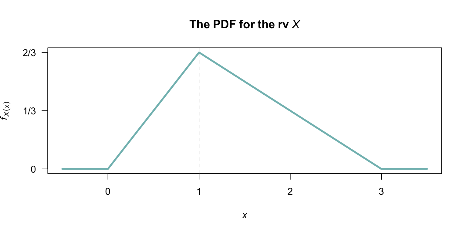
FIGURE 9.13: The probability density function for the random variable \(X\).

Exercise 9.25 Suppose the random variable \(X\) is defined as shown in Fig. 9.13.

1. Determine the distribution function for \(X\) (this was done in Exercise 9.24).
2. Find the probability density function for the random variable \(Z\), where \(Z = (X - 2)^2\).
3. Confirm that your probability density function for \(Z\) is a valid pdf.
4. Plot the probability density function of \(Z\).

Exercise 9.26 Let \(X_1, X_2, \ldots, X_n\) be independent positive random variables, and let \[ P = X_1 \cdot X_2 \cdots X_n = \prod_{i=1}^n X_i \] be their product.

1. Show that \(\log P = \sum_{i=1}^n \log X_i\), where \(P = \prod_{i=1}^n X_i\).
2. Hence show that \(P \sim \text{Log-normal}\!\left(\sum_{i=1}^n \mu_i,\, \sum_{i=1}^n \sigma_i^2\right)\).
3. Suppose \(X_1, X_2, \ldots, X_{10}\) are independent with \()\log X_i \sim N(0.2, 0.09)\) for each \(i\). Find the distribution of \(P = \prod_{i=1}^{10} X_i\) and hence find \(\Pr(P > \exp 3)\).

Exercise 9.27 Suppose the random variable \(X\) has the PDF \[ f_X(x) = (x + 1)/2\quad\text{for $-1 < x < 1$}. \]

1. Find the distribution function of \(X\).
2. Find the distribution function of \(Y = |X|\).
3. Hence find the probability density function of \(Y\).
4. Plot the PDF of both \(X\) and \(Y\),
5. Using the plot, explain why the PDF of \(Y\) Y has the shape it does, referring to the distribution of \(X\) and the transformation used.

---

Exercise 9.28 In this exercise, we revisit Exercise 7.46.

Suppose the finishing time \(T\) (in minutes) for marathon runners is modelled by \[ T\sim N(\mu, 36^2). \] Consider two runners (say, \(A\) and \(B\)) for whom \(\mu_A = 250\,\text{mins}\) and \(\mu_B = 280\,\text{mins}\). Assume the finishing times of the two runners are independent. The length of a marathon is \(42.195\,\text{km}\).

1. Show that the average speed (in \(\text{km}.\text{h}^{-1}\)) during the marathon is \(V = 60\times 42.195/T\).
2. Find the probability density function of the average speed for Runner A, \(V_A\).
3. Find the probability density function of the average speed for Runner B, \(V_B\).
4. Use R to simulate the probability density function of \(V_A - V_B\).

Exercise 9.29 Suppose that the radius (in metres) of oil spills \(R\) in marians and harboiurs from small boat leaks is \[ R \sim \text{Exponential}(\lambda). \] For one marina, \(\lambda = 0.2\) per metre.

1. Find the probability density function for the area of the oil spills.
2. Plot this PDF.
3. Use R to compute \(\Pr(A > 200)\).

Exercise 9.30 Suppose that bases for twelve-inch pizzas are made with a radius \(R\) (in inches). The manufacturing process restricts the minimum radius to \(11\) inches, and the maximum to \(13\) inches, with a mode of \(12\) inches: \[ f_R(r) = \begin{cases} (r - 11)/2 & \text{for $11\le r \le 12$};\\ (13 - r)/2 & \text{for $12 < r \le 13$.} \end{cases} \]

1. Find the probability density function for the area of the pizza base.
2. Plot this PDF.

---

Exercise 9.31 If a projectile (such as a cricket ball) is thrown directly up with velocity \(U\) (in \(\,\text{m}.sec^{-1}\), it reaches a maximum height of \(u^2/2g\), where \(g \approx 9.8m\sec^{-2}\) in acceleration due to gravity.

1. Suppose the initial velocity is distributed as \(U\sim N(15, 2^2)\). Find the probability density function of the maximum height of the projectile.
2. Suppose the initial velocity is distributed as \(U\sim \text{Gamma}(\text{shape} = 10, \text{scale} = 1.5)\). Find the probability density function of the maximum height of the projectile.
3. On the same plot, draw the pdf for both distributions.
4. Compute the mean height for each distribution.

---

Peter K. Dunn, Taryn Axelsen 2026: CC BY-NC-SA 4.0