8 Mixed distributions*
On completion of this chapter, you should be able to:
- recognise mixed random variables.
- recognise zero-modified distributions and compound Poisson–gamma models for modelling mixed random variables.
- know the basic properties of the above approaches.
- apply these approaches as appropriate to problem solving.
8.1 Introduction
Mixed random variables commonly occur in practice, in diverse applications such as insurance, agriculture, climatology, fisheries, etc. In most practical cases, a mixed random variable \(X\) has a discrete probability mass at \(X = 0\), and is also continuous for \(X > 0\). Examples include:
- Modelling insurance: some portfolios will have zero claims; however, when claims are made, the total claim amount has a positive continuous distribution.
- Modelling rainfall: some months may receive exactly zero rainfall; otherwise, the monthly rainfall has a continuous distribution.
- Modelling fish catch: some trawls will catch zero fish; other trawls, however, will catch a positive continuous mass of fish.
Continuous data with a discrete probability at zero can be modelled in various ways, depending on how the discrete probability at \(X = 0\) is modelled. Two approaches are considered in this chapter.
Zero-modified distributions (Sect. 8.2) treat the zeros as emerging from a two-step process. Step one is a binary process, that models whether the event of interest (i.e., an insurance claim is made; rainfall is recorded; fish are caught) occurs. Step two is a model for the continuous data of interest, conditional on the event of interest occurring.
The compound Poisson–gamma model (Sect. 8.3) generates zeros naturally from a single process: a zero count from the underlying Poisson distribution results in a zero response.
8.2 Zero-modified distributions
Zero-modified distributions assume a continuous distribution for positive continuous data, modified to have a discrete probability for \(X = 0\). The continuous distribution is sometimes an exponential distribution (Sect. 7.4), or more commonly a gamma (Sect. 7.5) or log-normal distribution (Sect. 7.6). Other distributions can also be used. Zero-modified distributions are also called zero-altered distributions or hurdle models.
8.2.1 Definitions
A zero-modified distributions treats zeros and positive values as arising from two separate processes. The first process is a binary model that determines whether an event occurs or not. The second process that describes the distribution of values, conditional on the values being positive. A zero-modified distribution is useful when the zero-generating process is believed to be distinct from the process driving variation among positive values; for example, whether a household buys alcohol is a different process than how much a household spends on alcohol if they do buy alcohol.
A zero-modified distribution treats the values of the random variable \(X\) as emerging from a two-step process. The first step uses a Bernoulli distribution (Sect. 6.3) to model a random variable \(Y\) that defines whether an event of interest occurs: \[ \Pr(Y) = \begin{cases} p & \text{if $Y = 0$; i.e., the event of interest does not occur;}\\ 1 - p & \text{if $Y = 1$; i.e., the event of interest does occur.} \end{cases} \] If the event does occur (i.e., conditional on \(X > 0\)), with probability \(1 - p\), then the continuous component is modelled using a probability density function \(f^+_X(x)\) defined for positive real values only (such as an exponential distribution, a gamma distribution or a log-normal distribution).
Definition 8.1 (Zero-modified distribution) A random variable \(X\) has a zero-modified distribution with continuous component \(f^+_X(x)\) if its probability function is \[ f_X(x) = \begin{cases} p & \text{if $x = 0$}\\ (1 - p)\cdot f^+_X(x) & \text{if $x > 0$,} \end{cases} \] where \(p = \Pr(X = 0) \in (0, 1)\) and \(f^+_X(x)\) is a probability density function defined for \(x > 0\) satisfying \(\int_0^\infty f^+_X(x)\,dx = 1\).
The corresponding distribution function is \[ F_X(x) = \begin{cases} 0 & \text{if $x < 0$}\\ p & \text{if $x = 0$}\\ p + (1-p)\cdot F^+_X(x) & \text{if $x > 0$.} \end{cases} \] Common choices for the continuous component \(f^+_X(x)\) include the exponential (Sect. 7.4), gamma (Sect. 7.5), and log-normal (Sect. 7.6) distributions.
In general, we write \(X \sim \text{ZM-$D$}(p, \dots)\), where \(D\) is any distribution on \((0, \infty)\) and the parameters of the distribution \(D\) are listed after \(p\). For example, \(X \sim \text{ZM-Gamma}(p, \alpha, \beta)\) specifies a zero-modified gamma distribution, where the \(\text{Gamma}(\alpha, \beta)\) distribution is used to model the continuous component.
Various zero-modified exponential distributions are shown in the visualisation below, for different values of \(\lambda\) and \(p\).
FIGURE 8.1: Zero-modified exponential distributions.
Various zero-modified gamma distributions are shown in the visualisation below, for different values of \(\alpha\), \(\beta\) and \(p\).
FIGURE 8.2: Zero-modified exponential distributions.
Example 8.1 (Zero-modified model) Consider the mixed random variable \(X\), with probability function \(f_X(x)\). Suppose that, when \(X > 0\), an exponential distribution is used to describe the distribution; that is \[ f^+_X(x) = \lambda \exp(-\lambda x)\quad\text{for $x > 0$}. \] Then, using \(p = 0.3\) and \(\lambda = 1/2\), the probability function of \(X\) is \[ f_X(x) = \begin{cases} 0.3 & \text{if $x = 0$}\\ 0.35\cdot \exp(-x/2) & \text{if $x > 0$.} \end{cases} \] Similarly, the distribution function of \(X\) is \[ F_X(x) = \begin{cases} 0 & \text{if $ x < 0$}\\ 0.3 & \text{if $x = 0$}\\ 0.7\cdot \left(1 - \exp(-x/2)\right) & \text{if $x > 0$.} \end{cases} \] The probability function and distribution function are shown in Fig. 8.3.
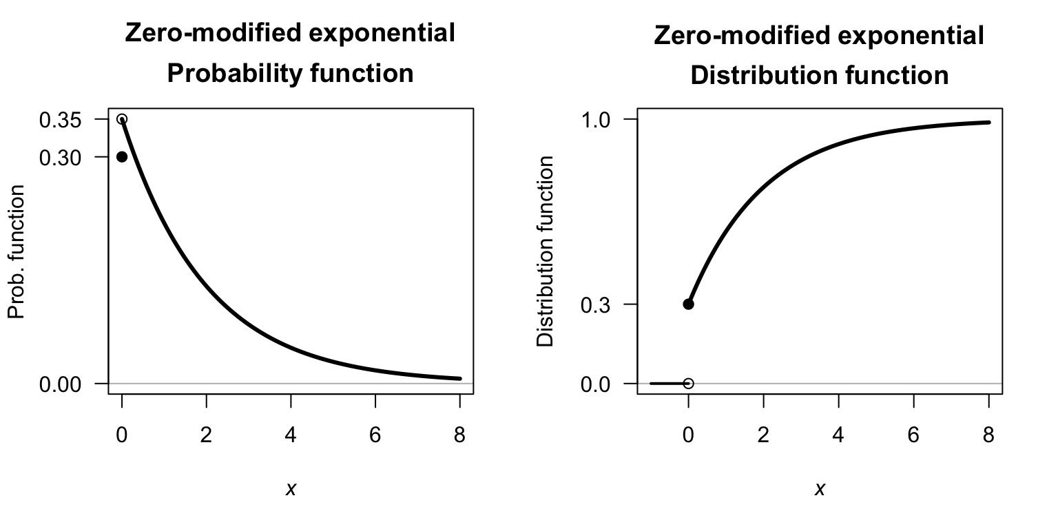
FIGURE 8.3: Zero-modified distributions, showing an exponential distribution for the continuous component.
8.2.2 Properties
The following are the basic properties of the zero-modified distributions.
Theorem 8.1 (Zero-modified distribution properties) If \(X\sim\text{ZM}(p)\) and \(\mu_c\) denotes \(\operatorname{E}[X\mid X > 0]\) (the expected value of the conditional distribution defined for \(X > 0\)) and \(\sigma^2_c = \operatorname{var}[X \mid X > 0]\), then
- \(\operatorname{E}[X] = (1 - p)\mu_c\).
- \(\operatorname{var}[X] = (1 - p) \sigma^2_c + p(1 - p)\mu_c^2\).
- \(M_X(t) = p + (1 - p)\cdot M_{X\mid X > 0}(t)\), where \(M_{X_c}(t)\) is the MGF of the conditional distribution \(X\mid X > 0\).
Proof. To compute the expected value of the random variable \(X\), first separate the discrete and continuous parts of the distribution: \[\begin{align*} \operatorname{E}[X] &= p\cdot \operatorname{E}[X\mid X = 0] + (1 - p)\cdot \operatorname{E}[X\mid X > 0]\\ &= (p\times 0) + (1 - p) \operatorname{E}[X\mid X > 0]\\ &= (1 - p) \mu_c, \end{align*}\] where \(\mu_c\) denotes \(\operatorname{E}[X\mid X > 0]\), the expected value of the (conditional) distribution defined for \(X > 0\). Similarly, \[ \operatorname{E}[X^2] = (p\times 0) + (1 - p) \operatorname{E}[X^2 \mid X > 0] = (1 - p)(\sigma_c^2 + \mu_c^2). \] Then, the variance of \(X\) is \[\begin{align*} \operatorname{var}[X] &= (1 - p)(\sigma^2_c + \mu^2_c) - (1 - p)^2\mu_c^2\\ &= (1 - p) \sigma^2_c + p(1 - p)\mu_c^2 \end{align*}\] where \(\sigma^2_c = \operatorname{var}[X \mid X > 0]\).
The same approach also gives the MGF as \[\begin{align*} M_X(t) &= p + (1 - p)\cdot M_{X_c}(t)\\ &= p + (1 - p)\cdot M_{X\mid X > 0}(t), \end{align*}\] where \(M_{X_c}(t)\) is the MGF of the conditional distribution \(X\mid X > 0\).
Further progress with these expressions requires knowing the distribution of \(X \mid X > 0\).
Example 8.2 (Zero-modified gamma distribution) Consider a random variable \(X\) such that \(p = 0.25\) (and hence \(\Pr(X = 0) = 0.25\)), and where the distribution when \(X > 0\) follows a gamma distribution (Sect. 7.5) having \(\alpha = 2\) and \(\beta = 1\), with the density function \[ f_X^{+}(x; \alpha, \beta) = f_{X\mid X > 0}(x; \alpha, \beta) = \frac{1}{\Gamma(2)} x \exp(-x) \quad\text{for $x > 0$}. \] For this gamma distribution, using results from Sect. 7.5, \(\mu_c = \operatorname{E}[X\mid X > 0] = \alpha\beta = 2\) and \(\sigma_c^2 = \operatorname{var}[X\mid X > 0] = \alpha\beta^2 = 2\). Then, the probability function for \(X\) is \[ f_{X}(x) = \begin{cases} 0.25 & \text{for $x = 0$}\\ 0.75 \times f_X^{+}(x; \alpha, \beta) & \text{for $x > 0$.} \end{cases} \] Then \[\begin{align*} \operatorname{E}[X] &= (1 - p)\cdot \mu_c = 0.75 \times 2 = 1.5\\ \operatorname{var}[X] &= (1 - p) \sigma_c^2 + p(1 - p)\mu_c^2 = (0.75\times 2) + (0.75\times 0.25\times 2^2) \approx 2.25. \end{align*}\] The probability function and distribution function are shown in Fig. 8.4.
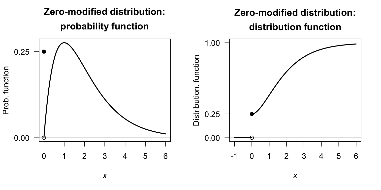
FIGURE 8.4: A zero-modified model, using a gamma distribution for the continuous component.
8.3 Compound Poisson–gamma distributions
8.3.1 Definition
A compound Poisson–gamma model generates the point mass at zero through a physically-motivated compound process. The model assumes that events occur according to a Poisson process, and each event contributes an independent gamma-distributed amount to the total. The observed variable \(Y\) is the sum of all the independent contributions. A compound Poisson–gamma distribution, therefore, is a Poisson sum of independent gamma distributions.
When the Poisson count is zero (i.e., when no events occur), the total is exactly zero, naturally producing the point mass without any separate modelling of zeros. When at least one event occurs, the sum of gamma random variables gives a continuous positive value. The compound Poisson–gamma distribution is a unified single-distribution model, and requires the compound Poisson–gamma story to be a plausible description of the data-generating process.
More specifically, suppose the number of events observed (a discrete random variable) is \(N\), such that \[\begin{equation} N \sim \text{Poisson}(\lambda). \tag{8.1} \end{equation}\] That is, an event occurs \(N\) times, where \(N\) follows a Poisson distribution. Given that \(N\) has a Poisson distribution, it follows (from Sect. 6.7) that \[ \Pr(N = 0) = \exp(-\lambda) \] is the probability that zero events are observed (i.e., \(N = 0\)). If, however, \(N > 0\), then for each \(i = 1, 2, \dots, N\), a continuous random variable \(Y_i\) is observed that follows a gamma distribution, such that \[ Y_i \sim \text{Gamma}(\alpha, \beta). \] where \(\alpha\) is the shape parameter and \(\beta\) is the scale parameter. If \(N = 0\), then no events \(Y_i\) are observed at all; however, if \(N > 0\) then \(N\) events are observed and \[ X = \sum_{i = 1}^N Y_i \] has a continuous distribution. Then, \[ X = \begin{cases} 0 & \text{if $N = 0$};\\ \sum_{i = 1}^N Y_i & \text{if $N > 0$}. \end{cases} \] By this definition \(X\) has a compound Poisson–gamma distribution (which are special cases of Tweedie distributions). The distribution of \(X\) has a probability mass at \(X = 0\) where \(\Pr(X = 0) = \Pr(N = 0) = \exp(-\lambda)\).
In general, the probability function for the compound Poisson–gamma distributions cannot be written in closed form, but instead are described by the MGF.
Definition 8.2 (Compound Poisson--gamma distribution) A random variable \(X\) has a compound Poisson–gamma distribution if its MGF is \[ M_X(t) = \exp\left\{ \lambda \left[ \left( \frac{\beta}{\beta - t}\right)^\alpha - 1\right]\right\} \quad \text{for $t < 1/\beta$} \] where \(\lambda > 0\), \(\alpha > 0\) is the shape parameter and \(\beta > 0\) is the scale parameter. We write \(X\sim \text{CPG}(\lambda, \alpha, \beta)\). The support is \(\{0\}\cup (0, \infty)\).
Various compound Poisson-gamma distributions are shown in the visualisation below, for different values of \(\lambda\), \(\alpha\) and \(\beta\).
FIGURE 8.5: Compound Poisson-gamma distributions.
Example 8.3 (Rainfall modelling) Consider monthly rainfall \(X\) at a given location. In any given month, \(N\) rainfall events may occur (and for some months, \(N\) may be zero) such that \[ N \sim \text{Poisson}(\lambda = 2.3). \] So, for example, that probability that a given month has no rainfall is \[ \Pr(N = 0) = \exp(-2.3) = 0.10, \] or about \(10\)%.
When a rainfall event does occur, the amount of rainfall is described by a gamma distribution \[ Y_i \sim \text{Gamma}(\alpha_i, 2), \] where \(\alpha_i\) may be different for each month \(i\).
Suppose \(\alpha_1 = 1.75\) in January and \(\alpha_6 = 0.3\) in June. The Poisson distribution remains the same for both months (Fig. 8.6, left panel), meaning that the distribution of the number of rainfall events is the same in January and in June. However, since the value of \(\alpha\) is different for each month, the distributions of the amount of rainfall in each rainfall event changes (Fig. 8.6, center panel). The distribution of total rainfall for the January and June rainfall using this model are shown in Fig. 8.6 (right panel).
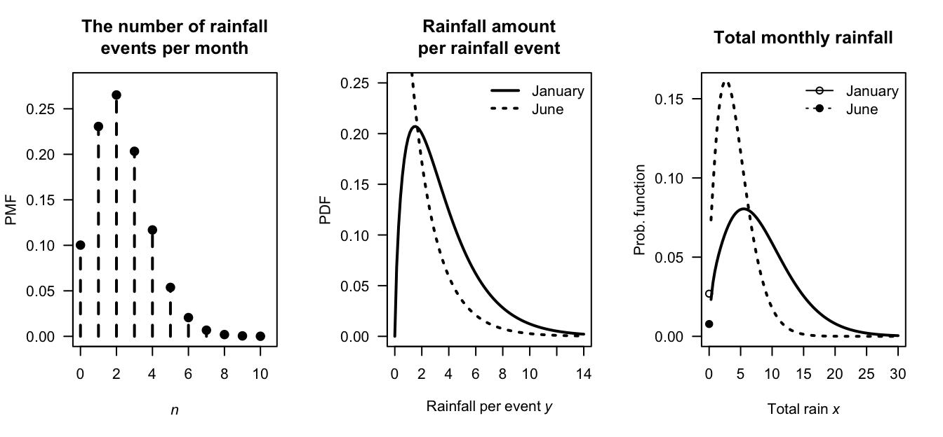
FIGURE 8.6: A compound Poisson–gamma model for rainfall. Left: the distribution of the number of rainfall events per month. Center: the distribution of rainfall per event for each month. Right: the distribution of the total rainfall for each month.
8.3.2 Properties
The following are the basic properties of compound Poisson–gamma distributions.
Theorem 8.2 (Compound Poisson--gamma distribution properties) If \(X\sim\text{CPG}(\lambda, \alpha, \beta)\) then:
- The expected value: \(\operatorname{E}[X] = \mu = \lambda\alpha\beta\).
- The variance: \(\operatorname{var}[X] = \lambda\alpha(\alpha + 1)\beta^2\).
- The probability of an exact zero: \(\Pr(X = 0) = \exp(-\lambda)\).
- The MGF is given in Def. 8.2.
- The conditional mean: \(\operatorname{E}[X\mid X > 0] = \lambda\alpha\beta/(1 - \exp(-\lambda))\).
- The reproductive property: If \(X_1\sim \text{CPG}(\lambda_1, \alpha, \beta)\) and \(X_2\sim\text{CPG}(\lambda_2, \alpha, \beta)\) independently, then \(X_1 + X_2 \sim\text{CPG}(\lambda_1 + \lambda_2, \alpha, \beta)\).
Proof. The proofs rely on the Laws of total expectation and variance (Sect. 10.11). The proof for the expected value appears in Example 10.31. The proof for the variance appears in Example 10.33. The proof of the MGF is given below. The proof of \(\operatorname{E}[X\mid X > 0]\) is Exercise 8.34. The proof of the reproductive property is Exercise 8.31).
The probability functions for the compound Poisson–gamma distribution cannot be written in closed form. However, the probability function can be expressed as an infinite sum (Dunn and Smyth 2005) or by inverting the MGF (Dunn and Smyth 2008), following the ideas in Sect. 5.6.5. Likewise, the distribution function has no closed form and must be evaluated using numerical methods (Dunn and Smyth 2026 (To appear)).
The probability function as an infinite series can be determined from the development of the compound Poisson–gamma distribution above. If \(N = 1\), which occurs with \(\Pr(N = 1) = \exp(-\lambda)\) (from the Poisson distribution), then, \(X = Y\) has the \(\text{Gamma}(\alpha, \beta)\) distribution. That is, \[ f_{X\mid N = 1}(x) = \frac{1}{\Gamma(\alpha)\,\beta^{\alpha}} x^{\alpha -1}\exp(-x/\beta) \quad \text{for $x > 0$}. \]
If \(N = 2\), then, \(X = Y_1 + Y_2\), where \(Y_i \sim\text{Gamma}(\alpha, \beta)\) for \(i = 1, 2\). This means that \(X \sim \text{Gamma}(2\alpha, \beta)\) (Exercise 9.3; Sect. 7.5.2). That is, \[ f_{X\mid N = 2} (x) = \frac{1}{\Gamma(2\alpha)\,\beta^{2\alpha}} x^{2\alpha -1}\exp(-x/\beta) \quad \text{for $x > 0$}. \]
More generally, if \(N = n\), then \(X = Y_1 + Y_2 + \cdots + Y_n\), and so \(X \sim\text{Gamma}(n\alpha, \beta)\), so that \[ f_{X\mid N = n} (x) = \frac{1}{\Gamma(n\alpha)\, \beta^{n\alpha}} x^{n\alpha -1}\exp(-x/\beta) \quad \text{for $x > 0$}. \]
Then, conditioning on the value of \(N\), \[\begin{align*} f_X(x) &= \sum_{n = 1}^\infty \Pr(N = n) \cdot f_{X\mid N = n}(x)\\ &= \sum_{n = 1}^\infty \frac{\exp(-\lambda)\lambda^n}{n!} \cdot \frac{1}{\Gamma(n\alpha)\,\beta^{n\alpha}} x^{n\alpha -1}\exp(-x/\beta)\\ &= \exp(-\lambda - x/\beta) \sum_{n = 1}^\infty \frac{\lambda^n}{n!} \frac{x^{n\alpha - 1}}{\Gamma(n\alpha)\, \beta^{n\alpha}} \end{align*}\] for \(x > 0\). In addition, of course, \[ \Pr(X = 0) = \exp(-\lambda). \]
Even though the probability function has no closed form, the MGF is reasonably simple. To find the MGF, first consider the value of \(N\) as fixed; then, \(X = Y_1 + Y_2 + \cdots + Y_N\) the MGF of \(X\) is \[ M_{X\mid N}(t) = \operatorname{E}[\exp(tX)\mid N]. \] Since the MGF of a sum of independent random variables is the product of their MGFs (Theorem 5.9), we can assume that \(N\) takes some specific value \(n\) and write \[\begin{align*} M_{X\mid N}(t) &= \operatorname{E}\left[ \exp\big(t(Y_1 + Y_2 + \cdots + Y_n)\big)\right] \\ &= \prod_{i = 1}^n \operatorname{E}[\exp(t Y_i)] \\ &= M_Y(t)^n \end{align*}\] So the MGF of \(X\) (rather than \(X\mid N\) as above) is \[\begin{align*} M_X(t) &= \operatorname{E}\left[ \operatorname{E}[ \exp(tX) \mid N]\right] \\ &= \operatorname{E}\left[ M_{X\mid N}(t)\right] \\ &= \operatorname{E}\left[ M_Y(t)^N\right]. \end{align*}\] Substituting the MGF of a \(\text{Gamma}(\alpha, \beta)\) random variable, \(M_Y(t) = \left(\frac{1}{1 - \beta t}\right)^{\!\alpha}\), and then applying the MGF of a \(\text{Poisson}(\lambda)\) random variable, \(M_N(s) = \exp\{\lambda(s - 1)\}\) with \(s = M_Y(t)\), gives \[ M_X(t)=\exp\!\left\{\lambda\left[\Big(\frac{1}{1 - \beta t}\Big)^{\!\alpha}-1\right]\right\},\qquad\text{for $t < 1/\beta$}. \]
From the MGF we can deduce \[\begin{align*} \operatorname{E}[X] &= \lambda\alpha\beta\\ \operatorname{var}[X] &= \lambda\alpha\beta^2(\alpha + 1). \end{align*}\]
Example 8.4 (Poisson--gamma distribution) Suppose \[ N\sim\text{Poisson}(\lambda = 3) \quad\text{and}\quad Y_i \sim\text{Gamma}(\alpha = 1/2, \beta = 2/3) \] (where \(\beta\) is the scale parameter). The mean and variance of \(X\) is \[\begin{align*} \operatorname{E}[X] &= \lambda\alpha\beta = 3\times \frac{1}{2}\times\frac{2}{3} = 1;\\ \operatorname{var}[X] &= \lambda\alpha(\alpha + 1)\beta^2 = 3\times \left(\frac{1}{2}\times \frac{3}{2}\right)\left(\frac{2}{3}\right)^2 = 1. \end{align*}\] Furthermore, from Equation (8.1), \[ \Pr(X = 0) = \exp(-\lambda) = 0.0498. \]
8.3.3 The mean–variance parameterisation
The compound Poisson–gamma probability function defined in Def. 8.2 has three parameters: \(\lambda\) (from the underlying Poisson distribution) and \(\alpha\) and \(\beta\) (from the underlying gamma distribution).
The probability function can also be written using the parameters \(\mu\), \(\phi\) and \(\xi\), where \[ \xi = 1 + \frac{1}{\alpha + 1}; \qquad \operatorname{E}[X] = \mu = \lambda\alpha\beta; \qquad \phi = \frac{\lambda\alpha(\alpha + 1)\beta^2}{\mu^\xi}, \] when \[\begin{equation} \operatorname{var}[X] = \mu^\xi. \tag{8.2} \end{equation}\] Distributions with the mean–variance relationship shown in Eq. (8.2) are defined for \(\xi = (-\infty, 0] \cup [1, \infty)\) and are called Tweedie distributions. The compound Poisson–gamma distributions are a special case of the Tweedie distributions, where \(1 < \xi < 2\). The compound Poisson–gamma parameters (\(\lambda\), \(\alpha\), \(\beta\)) describe how the data are generated, while the Tweedie parameters (\(\mu\), \(\phi\), \(\xi\)) describe the relationship between the mean and variance of the same distribution.
Accurate evaluation and plotting of the compound Poisson–gamma distributions can be facilitated by installing, loading and using the tweedie package in R (Dunn 2026), which uses the \((\mu, \phi, \xi)\) parameterisation.
The four R functions for working with the compound Poisson–gamma distributions have the form [dpqr]tweedie(., xi, mu, phi) (see App. E):
-
dtweedie(x, xi, mu, phi)computes the PDF at \(X = {}\)x; -
ptweedie(q, xi, mu, phi)computes the CDF at \(X = {}\)q; -
qtweedie(p, xi, mu, phi)computes the quantile for cumulative probabilityp; and -
rtweedie(n, xi, mu, phi)generatesnrandom numbers,
where mu\({} = \mu\), phi\({} = \phi\), xi\({} = \xi\).
Example 8.5 (Plotting compound Poisson--gamma distributions) Plotting compound Poisson-gamma distribution is achieved using the tweedie package in R; the function tweedie_plot() makes this easy (Fig. 8.7):
mu <- 1
phi <- 1
xi <- 1.5
x <- seq(0, 5,
         length = 200)

library(tweedie)
tweedie_plot(x, xi = xi, mu = mu, phi = phi,
             plot_args = list(las = 1),   # Horizontal axis labels
             line_args = list(lwd = 3) )  # Thicker lines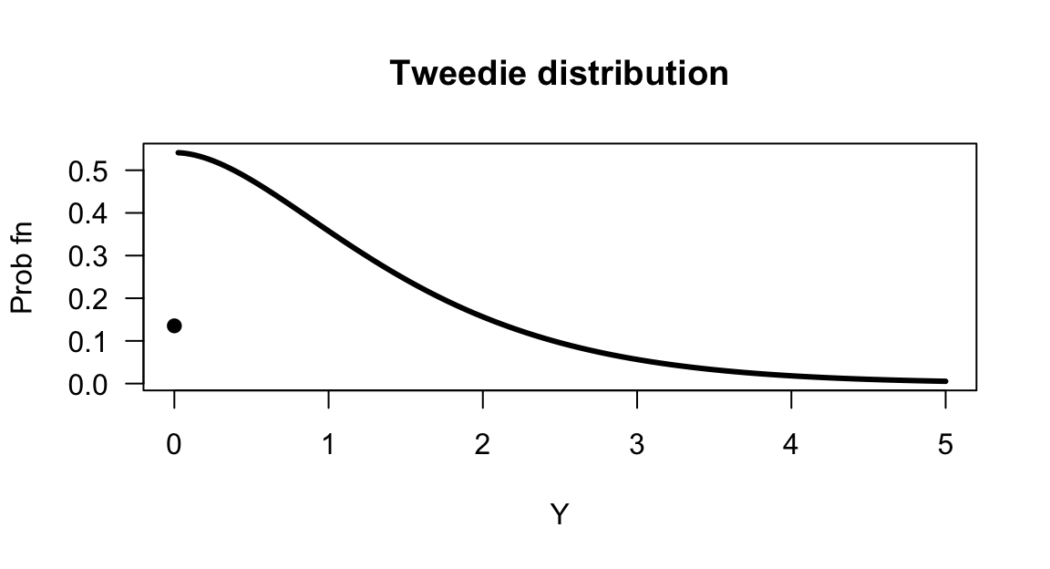
FIGURE 8.7: A compound Poisson–gamma distribution.
8.4 Summary of models
The zeros in a compound Poisson–gamma distributions are a natural outcome of the same process used to generate the non-zero values; a zero occurs when the Poisson count of contributions is zero. If a physical argument can be provided that the observed value is the sum of a random number of independent gamma-distributed contributions, a compound Poisson–gamma distribution may be an appropriate model.
In contrast, a zero-modified distribution model treats zeros and positive values as structurally distinct, potentially generated by different processes: a separate model governs whether an observation is zero, and another governs an observation’s magnitude given it is positive.
| Zero-modified | Poisson-Gamma | |
|---|---|---|
| Zeros | Different process | No events occurred |
| Parameters | Two separate models | One unified model |
| Interpretation | Very natural | Requires physical story |
| Flexibility | High | Moderate |
| Uses | Healthcare spend | Insurance, rainfall |
Example 8.6 (Insurance modelling) Insurance companies have some days when zero claims are lodged, but most days record numerous claims, each of which are for positive, right-skewed amounts.
A compound Poisson–gamma model could be considered. The daily claim total is the aggregate of a random number of individual claim events (accidents or incidents), each generating a gamma-distributed payout amount. A zero-claim amount occurs when no claim events arrive. The same process (i.e., policy-holders having incidents) generates both zeros and positive values.
A zero-modified distribution could also be considered. First, a binary process determines whether any claim is filed (perhaps driven by seasonal risk, policy-holder behaviour, or reporting thresholds). Conditional on a claim occurring, the total payout follows a gamma distribution. The zero (no-claim day) and positive values are structurally different; a no-claim day is not just ‘zero incidents happened’, but may reflect under-reporting, policy excesses, or deliberate non-filing.
8.5 Simulation
8.5.1 Simulating mixed distributions
Simulating mixed distribution is usually more involved than sampling for discrete and continuous distributions, as functions for generating random numbers are not always easily available for mixed distributions. However, an understanding of the process behind the mixed random variable can be used to generate random numbers.
For example, to generate data from a zero-modified exponential distribution with \(p = 0.3\) and \(\lambda = 5\), we can first simulate whether or not the continuous event will occur using a Bernoulli distribution:
n <- 10                             # How many random numbers to generate
is_zero <- rbinom(n,                # Generate three random numbers...
                  size = 1,         # ... from 0 and 1 (i.e., Bernoulli)....
                  prob = 0.3)       # ... with prob = 0.3
is_zero
#>  [1] 0 0 0 1 0 0 0 0 1 0
where_zero <- (is_zero == 0)       # Where the zeros are in the vector
where_pos  <- (is_zero == 1)       # Where the positive values are located
Then, when the random value is \(1\), generate a random exponential value:
n_pos <- sum(where_pos)            # How many values are non-zero?
cont_values <- rexp(n_pos,         # For each non-zero value use rexp()...
                    rate = 5)      # ... with rate = 5

###   Now combine zeros and positive values
rnos <- numeric(n)                 # Create a vector to hold all random numbers
rnos[where_pos] <- cont_values     # Place continuous values where ones occur
rnos[where_zero] <- 0              # Please zeros where zeros occur

rnos
#>  [1] 0.00000000 0.00000000 0.00000000 0.04366418 0.00000000
#>  [6] 0.00000000 0.00000000 0.00000000 0.24204531 0.00000000
If the random numbers are used frequently, using a function is easier:
rzm_exp <- function(n, lambda, p0) {
  is_zero <- rbinom(n,            # Generate n Bernoulli random numbers
                    size = 1,     # size = 1 ensure Bernoulli random numbers
                    prob = p0)    # Use the given probability
  n_exp <- sum(!is_zero)          # This counts how many random numbers are not-zero
  out <- numeric(n)               # Prepare a vector to hold the random numbers
  out[!is_zero] <- rexp(n_exp,    # For each non-zero value, generate using rexp()
                        rate = lambda)
  out                             # Return the random numbers
}

rzm_exp(10, lambda = 5, p0 = 0.3)
#>  [1] 0.72875901 0.28999387 0.15075784 0.71742090 0.00000000
#>  [6] 0.00178837 0.21586269 0.16695096 0.15179528 0.34190619
Clearly, the function needs to be adapted for other zero-modified distributions, by using rgamma() or rlnorm() in place of rexp().
For example:
rzm_gamma <- function(n, shape, scale, p0) {
  is_zero <- rbinom(n,            # Generate n Bernoulli random numbers
                    size = 1,     # size = 1 ensure Bernoulli random numbers
                    prob = p0)    # Use the given probability
  n_gm <- sum(!is_zero)           # This counts how many random numbers are not-zero
  out <- numeric(n)               # Prepare a vector to hold the random numbers
  out[!is_zero] <- rgamma(n_gm,   # For each non-zero value, generate using rgamma()
                          shape = shape,
                          scale = scale)
  out
}

rzm_gamma(10, shape = 2, scale = 1.5, p0 = 0.3)
#>  [1] 0.0000000 1.1704544 8.0788593 3.5309439 1.2805347 3.2595247
#>  [7] 3.2504976 0.2792154 1.1998931 0.0000000
Similarly, random numbers from a compound Poisson–gamma distribution can be generated by understanding the process. This time, we write a function directly:
rcpg_first <- function(n, lambda, alpha, beta) {
  N <- rpois(n,                       # For each n, N is how many events occur...
             lambda = lambda)         # ... based on the Piosson mean (lambda)
  out <- numeric(n)                   # Prepare a vector to hold the random numbers
  for (i in which(N > 0)) {           # If i is greater than zero...
    out[i] <- sum(rgamma(N[i],        # ... add up that many gamma random numbers
                         shape = alpha,
                         scale = beta))
  }
  out
}

rcpg_first(10, lambda = 1, alpha = 1.25, beta = 5)
#>  [1]  0.000000  2.463543  2.872342  0.000000  6.401697  0.000000
#>  [7] 14.722016  0.000000  0.000000  0.000000
The function can be made more efficient (especially for generating a large number of compound Poisson–gamma random numbers) using that the sum of \(k\) independent \(\text{Gamma}(\alpha, \beta\)) distribution is a \(\text{Gamma}(k\alpha, \beta)\) distribution (Exercise 9.3):
rcpg <- function(n, lambda, alpha, beta) {
  N <- rpois(n,                       # For each sim n, N is how many events occur...
             lambda = lambda)         # ... based on the Poisson mean (lambda)
  out <- numeric(n)                   # Prepare a vector to hold the random numbers
  pos <- N > 0                        # pos is TRUE if N is larger than zero
  out[pos] <- rgamma(sum(pos),        # Where N>0, generate gamma random numbers
                     shape = N[pos] * alpha,   # Note: Gamma(k*alpha, beta)
                     scale = beta)
  out
}
rcpg(10, lambda = 1, alpha = 1.25, beta = 5)
#>  [1] 6.822064 1.434700 0.000000 8.236198 7.321114 8.783520
#>  [7] 2.041468 4.808624 0.000000 0.000000
8.5.2 Example: rainfall
Consider modelling monthly rainfall at a certain location for one specific month each year. Monthly rainfall is a mixed random variable: some months record exactly zero rainfall, while months in which rain falls have a continuous positive amount of rain recorded. Both zero-modified models (e.g., Stern and Coe (1984)) and compound Poisson–gamma distributions (e.g., Yunus et al. (2017)) can be used to model rainfall.
Suppose the monthly rainfall (in mm) \(R\) is modelled at a given location for a certain month, where about \(15\)% of months record zero rainfall; then \(\Pr(R = 0) = 0.15\). In addition, suppose the mean of the monthly rainfall is \(\operatorname{E}[R] = \mu = 8.5\,\text{mm}\), and the variance of the monthly rainfall is \(\operatorname{var}[R] = 56\,\text{mm}^2\).
For the zero-modified distribution, set \(p = 0.15\) for the probability of no rainfall; then, the probability that rain is recorded is \(1 - p = 0.85\). For the positive rainfall component, suppose first that rainfall amounts follow an exponential distribution with rate \(\lambda\). Since \(\operatorname{E}[R \mid R > 0] = 1/\lambda = 10\), we have \(\lambda = 0.1\). The zero-modified model is then (Fig. 8.8): \[ f_R(r) = \begin{cases} 0.15 & \text{for $r = 0$} \\ 0.85 \times 0.1\, \exp(-0.1r) & \text{for $r > 0$}. \end{cases} \]
pi0   <- 0.15          # P(R = 0)
mu_p  <- 10            # E[R | R > 0] = 10mm
num_sims <- 1000       # Number of simulations

# --- Zero-modified exponential ---
p        <- 1 - pi0
lambda   <- 1 / mu_p

Rain_zme <- rzm_exp(num_sims, lambda = 1/mu_p, p0 = pi0)

pData_zme <- mean(Rain_zme == 0)
theo_var_zme <- (1 - pi0) * (1/lambda)^2 + pi0 * (1 - pi0) * (1/lambda)^2
cat("Theoretical P(R = 0):  ", pi0, "\n",
    "Simulated P(R = 0):    ", round(mean(Rain_zme == 0), 3), "\n\n",
    "Theoretical E[R]:      ", (1 - pi0) * (1/lambda), "\n",
    "Simulated E[R]:        ", round(mean(Rain_zme), 3), "\n",
    "Theoretical Var[R]:    ", theo_var_zme, "\n",
    "Simulated Var[R]:      ", round(var(Rain_zme), 3), "\n")
#> Theoretical P(R = 0):   0.15
#>  Simulated P(R = 0):     0.147
#>
#>  Theoretical E[R]:       8.5
#>  Simulated E[R]:         8.233
#>  Theoretical Var[R]:     97.75
#>  Simulated Var[R]:       89.271
The zero-modified exponential distribution is a convenient starting point, but imposes a monotonically decreasing density on the positive part, which may be unrealistic; observed rainfall amounts often have a mode above zero. A gamma distribution for the positive part is more flexible, allowing a range of shapes, and is generally preferred in practice. The values of \(\alpha\) and \(\beta\) can be chosen to match the (unconditional) mean \(\mu^+ = 8.5\) and the (unconditional) variance \(\operatorname{var}[R] = 56\). Then \[\begin{align*} \operatorname{E}[R] &= (1 - p_0)\alpha\beta = 8.5, \text{and}\\ \operatorname{var}[R] &= (1 - p_0)\alpha\beta^2 + p_0(1 - p_0)(\alpha\beta)^2 = 56. \end{align*}\] Substituting \(\alpha\beta = 8.5/0.85 = 10\) into the variance equation and some algebra gives \[ \alpha \approx 1.965\quad\text{and}\quad\beta \approx 5.088. \]
# --- Zero-modified gamma ---
mu_c       <- mu_p                        # E[R | R > 0] = 10
target_var <- 56                          # Var[R] unconditional
# Solve: (1-pi0)*mu_c*scale + pi0*(1-pi0)*mu_c^2 = target_var
scale <- (target_var - pi0 * (1 - pi0) * mu_c^2) / ((1 - pi0) * mu_c)  # = 5.088
shape <- mu_c / scale                                                     # = 1.965

Rain_zmg   <- rzm_gamma(num_sims,
                     shape = shape,
                     scale = scale,
                     p0 = pi0)
theo_var_zmg <- (1 - pi0) * shape * scale^2 +
                pi0 * (1 - pi0) * (shape * scale)^2

pData_zmg <- mean(Rain_zmg == 0)
cat("Theoretical P(R = 0):  ", pi0, "\n",
    "Simulated P(R = 0):    ", round(mean(Rain_zmg == 0), 3), "\n\n",
    "Theoretical E[R]:      ", (1 - pi0) * shape * scale, "\n",
    "Simulated E[R]:        ", round(mean(Rain_zmg), 3), "\n",
    "Theoretical Var[R]:    ", theo_var_zmg, "\n",
    "Simulated Var[R]:      ", round(var(Rain_zmg), 3), "\n")
#> Theoretical P(R = 0):   0.15
#>  Simulated P(R = 0):     0.147
#>
#>  Theoretical E[R]:       8.5
#>  Simulated E[R]:         8.404
#>  Theoretical Var[R]:     56
#>  Simulated Var[R]:       51.344
For the compound Poisson–gamma model, monthly rainfall is the aggregate of a random number \(N \sim \text{Poisson}(\lambda)\) of independent rainfall events, each contributing a gamma-distributed amount (e.g., Yunus et al. (2017)). The zero probability is \(\Pr(R = 0) = \exp(-\lambda)\), so matching \(\Pr(R = 0) = 0.15\) gives \[ \lambda = -\log(0.15) \approx 1.89712. \] This leaves two free parameters: \(\alpha\) and \(\beta\) of the gamma distribution. Since \(\lambda\alpha\beta = 8.5\) and \(\lambda\alpha\beta^2(\alpha + 1) = 56\), some algebra gives \[ \alpha \approx 2.127\quad\text{and}\quad\beta \approx 2.107. \]
cat("Theoretical P(R = 0):  ", pi0, "\n",
    "Simulated P(R = 0):    ", round(mean(Rain_cpg == 0), 3), "\n\n",
    "Theoretical E[R]:      ", mu_R, "\n",
    "Simulated E[R]:        ", round(mean(Rain_cpg), 3), "\n",
    "Theoretical Var[R]:    ", round(theo_var_cpg, 3), "\n",
    "Simulated Var[R]:      ", round(var(Rain_cpg), 3), "\n")
#> Theoretical P(R = 0):   0.15
#>  Simulated P(R = 0):     0.135
#>
#>  Theoretical E[R]:       8.5
#>  Simulated E[R]:         8.611
#>  Theoretical Var[R]:     56
#>  Simulated Var[R]:       55.205
The empirical probability functions from each model are shown in Fig. 8.8. The zero-modified expinential distribution looks different than the other empirical probability functions, as it is a two-parameter distribution rather than a three-parameter distribution so has less flexibility.
![The empirical probability functions for rainfall from $1000$ simulations, each with $\Pr(R) = 0.15$, $\operatorname{E}[R] = 8.5\mms$ and $\operatorname{var}[R] = 56\mms^2$ (apart from the zero-modified exponential). Left:a zero-modified exponential distribution. Centre: zero-modified gamma distribution. Right: compound Poisson--gamma distribution.](08-MixedDistributions_files/figure-html/MixedRainEmp-1.png)
FIGURE 8.8: The empirical probability functions for rainfall from \(1000\) simulations, each with \(\Pr(R) = 0.15\), \(\operatorname{E}[R] = 8.5\,\text{mm}\) and \(\operatorname{var}[R] = 56\,\text{mm}^2\) (apart from the zero-modified exponential). Left:a zero-modified exponential distribution. Centre: zero-modified gamma distribution. Right: compound Poisson–gamma distribution.
Simulated rainfall sequences of this kind are rarely an end in themselves. In agriculture, simulated monthly rainfall feeds into crop yield models, where the distribution of yields (and particularly the probability of drought) is of direct interest. In hydrology, simulated rainfall drives runoff and reservoir models. In forestry, rainfall simulations inform fire risk assessments. In each case, the goal is to propagate uncertainty in rainfall through to uncertainty in a downstream quantity, which is difficult or impossible to do analytically but straightforward via simulation once a model for \(R\) has been specified and fitted.
cat("Estimated drought probability (R < 5mm):\n",
    "- using ZM-exponential model:",
    round(mean(Rain_zme < 5), 3), "\n",
    "- using ZM_Gamma model:",
    round(mean(Rain_zmg < 5), 3), "\n",
    "- using CP-G model:",
    round(mean(Rain_cpg < 5), 3), "\n")
#> Estimated drought probability (R < 5mm):
#>  - using ZM-exponential model: 0.488
#>  - using ZM_Gamma model: 0.357
#>  - using CP-G model: 0.376
8.5.3 Example: workplace injury costs
Workplace injuries impose direct costs on employers through medical treatment, rehabilitation, and lost productivity. Some work days have no injuries, and hence zero cost. On other days, one or more injuries may occur, generating a positive total cost. Daily injury cost is a mixed random variable.
Suppose daily injury costs (in thousands of dollars) \(C\) are modelled as \[ f_C(c) = \begin{cases} p & \text{for $c = 0$} \\ (1 - p) \cdot f^+_C(c) & \text{for $c > 0$}, \end{cases} \] where \(p = \Pr(C = 0) = 0.70\) (i.e., injury-free days are common) and the positive component \(f^+_C(c)\) follows a \(\text{Gamma}(\alpha = 2, \beta = 5)\) distribution. Hence, the mean cost is $10,000 on days when injuries do occur. The unconditional mean daily cost is therefore \[ \operatorname{E}[C] = (1 - p) \cdot \alpha\beta = 0.30 \times 10 = \$3\,000. \]
We can simulate \(n = 10\,000\) days of operation:
n_days  <- 10000
p0      <- 0.70          # P(C = 0): probability of injury-free day
alpha   <- 2             # Gamma shape
beta    <- 5             # Gamma scale: E[C | C > 0] = alpha * beta = 10

injury_day <- rbinom(n_days, size = 1, prob = 1 - p0)
C <- numeric(n_days)
pos <- injury_day == 1
C[pos] <- rgamma(sum(pos), shape = alpha, scale = beta)
We can verify the simulated properties against their theoretical values:
theo_mean <- (1 - p0) * alpha * beta
theo_var  <- (1 - p0) * alpha * beta^2 + p0 * (1 - p0) * (alpha * beta)^2

results <- c(
  "Theoretical P(C = 0)" = p0,
  "Simulated P(C = 0)"   = round(mean(C == 0), 3),
  "Theoretical E[C]"     = theo_mean,
  "Simulated E[C]"       = round(mean(C), 3),
  "Theoretical Var[C]"   = round(theo_var, 2),
  "Simulated Var[C]"     = round(var(C), 2)
)
print(results)
#> Theoretical P(C = 0)   Simulated P(C = 0)     Theoretical E[C]
#>                0.700                0.701                3.000
#>       Simulated E[C]   Theoretical Var[C]     Simulated Var[C]
#>                2.955               36.000               36.140
The model can be used to find answers to practical questions. For example, what is the distribution of daily costs?
pData <- mean(C == 0)
x_seq <- seq(0.01, max(C), length.out = 500)
cont_dens <- (1 - p0) * dgamma(x_seq, shape = alpha, scale = beta)

par(mfrow = c(1, 2))

plot(x_seq, cont_dens,
     type = "l",
     lwd = 2,
     xlim = c(-1, 60),
     ylim = c(0, pData * 1.2),
     las  = 1,
     main = "Daily injury costs",
     xlab = "Cost ($000s)",
     ylab = "Probability / Defective density")
#segments(x0 = 0, y0 = 0, x1 = 0, y1 = pData,
#         lwd = 3, col = "steelblue")
points(x = 0,
       y = pData,
       pch = 19,
       cex = 1.25)
text(x = 1,
     y = pData,
     labels = paste0("P(C = 0) = ", round(pData, 2)),
     pos = 4,
     cex = 0.9)

###

plot(x_seq, cont_dens,
     type = "l",
     lwd = 2,
     xlim = c(-1, 60),
     las  = 1,
     main = "Daily injury costs\nwhen injuries reported",
     xlab = "Cost ($000s)",
     ylab = "Conditional density")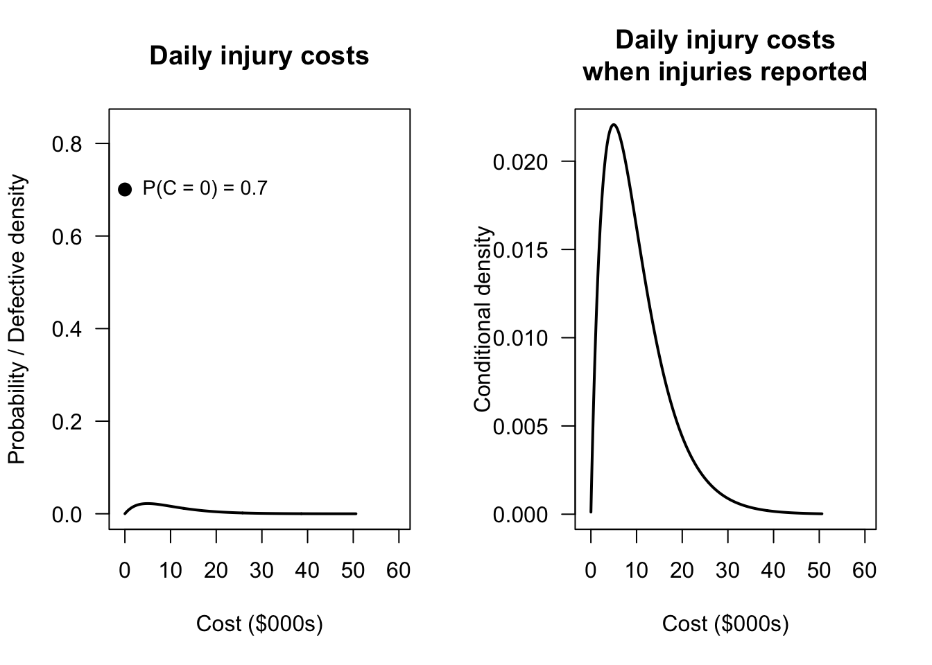
FIGURE 8.9: Distribution of daily injury costs. The point shows the probability mass at zero (injury-free days); the histogram shows the distribution of costs on injury days, scaled by \((1-p)\).
The model also can be used to find answers to questions that are difficult or impossible to answer analytically. One question is: what is the distribution of total annual costs?
Annual cost is the sum of \(250\) daily costs (assuming \(250\) working days per year). The distribution of this sum is analytically intractable; it is a compound distribution mixing a point mass at zero with a continuous component. This is straightforward using simulation:
n_sims       <- 10000
annual_costs <- replicate(n_sims, {
  days <- rbinom(250, size = 1, prob = 1 - p0)
  {pos <- days == 1
    c_days <- numeric(250)
    c_days[pos] <- rgamma(sum(pos), shape = alpha, scale = beta)
    sum(c_days)}
  })

cat("Simulated mean annual cost ($000s):  ",
    round(mean(annual_costs), 1), "\n",
    "Theoretical mean annual cost ($000s):",
    250 * (1 - p0) * alpha * beta, "\n\n",
    "Simulated sd annual cost ($000s):    ",
    round(sd(annual_costs), 1), "\n")
#> Simulated mean annual cost ($000s):   750.9
#>  Theoretical mean annual cost ($000s): 750
#>
#>  Simulated sd annual cost ($000s):     95.3
We could also ask: what premium should an insurer charge to cover annual costs with 95% probability?
The insurer needs the 95th percentile of annual costs. Quantile like this are easy to extract from simulations, but analytically intractable:
premium_95 <- quantile(annual_costs, 0.95)
cat("95th percentile of annual costs ($000s):",
    round(premium_95, 1), "\n",
    "This is", round(premium_95 / mean(annual_costs), 2),
    "times the mean annual cost.\n")
#> 95th percentile of annual costs ($000s): 910.5
#>  This is 1.21 times the mean annual cost.
Suppose the employer holds a monthly reserve of $50{,}000. What is the probability that costs in any single month exceed a fixed reserve?
The probability that monthly costs exceed this reserve is:
n_sims        <- 10000
monthly_costs <- replicate(n_sims, {
  days <- rbinom(21, size = 1, prob = 1 - p0)   # ~21 working days per month
  {pos <- days == 1
   c_days <- numeric(21)
   c_days[pos] <- rgamma(sum(pos), shape = alpha, scale = beta)
   sum(c_days)}}
  )

cat("P(monthly costs > $50,000):",
    round(mean(monthly_costs > 50), 3), "\n")
#> P(monthly costs > $50,000): 0.653
How sensitive is the 95th percentile premium to the probability of an injury-free day? As \(p\) increases (safer workplace), how does the required premium change? This sensitivity analysis is immediate via simulation, but otherwise would require re-deriving the entire distribution analytically for each value of \(p\):
p_seq    <- seq(0.50, 0.95, by = 0.05)
pct_95   <- numeric(length(p_seq))

for (j in seq_along(p_seq)) {
  p_j   <- p_seq[j]
  costs <- replicate(5000, {
    days <- rbinom(250, size = 1, prob = 1 - p_j)
    C_days <- numeric(250)
    C_days[days == 1] <- rgamma(sum(days == 1), shape = alpha, scale = beta)
    sum(C_days)
  })
  pct_95[j] <- quantile(costs, 0.95)
}

plot(p_seq, pct_95,
     type = "b", pch = 19, lwd = 2,
     col  = ColourSolid,
     las  = 1,
     xlab = expression("P(injury-free day) " ~ italic(p)),
     ylab = "95th percentile annual cost ($000s)",
     main = "Premium sensitivity to workplace safety")
abline(h = premium_95,
       lty = 2,
       col = ColourLightOpaque)
text(x    = 0.51,
     y    = premium_95 + 2,
     labels = paste0("Baseline (p = ", p0, ")"),
     adj  = 0, cex = 0.85, col = "gray40")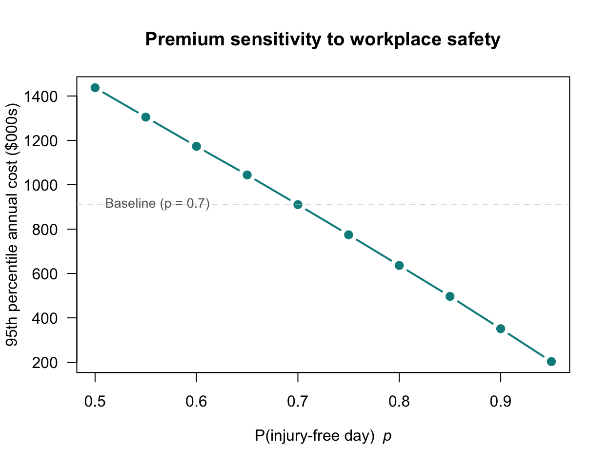
FIGURE 8.10: The 95th percentile of annual costs as a function of the probability of an injury-free day \(p\). As the workplace becomes safer (larger \(p\)), the required premium falls.
These simulations illustrate a key strength of the mixed distribution framework: once a model for \(C\) has been specified, uncertainty can be propagated through to any downstream quantity of interest (e.g., annual totals, percentiles, reserve adequacy) without requiring any additional analytical derivation.
8.6 Exercises
Selected answers appear in Sect. F.7.
Exercise 8.1 A rainfall gauge has a physical capacity of \(50\,\text{mm}\). When \(X > 50\), the gauge overflows, and is recorded as \(Y = 50\). Assume \(X \sim \text{Exponential}(\text{rate} = 1/20)\), where \(X\) is the monthly rainfall at a given weather station.
- Is \(X\) a discrete, continuous or mixed random variable? Explain.
- Define the support for \(X\).
- Define \(Y\) in terms of \(X\).
- Define the support for \(Y\).
- Is \(Y\) a discrete, continuous, or mixed random variable? Explain.
- Sketch the probability function of \(Y\), showing any point masses.
- Write down the cumulative distribution function of \(Y\).
- Sketch the distribution function of \(Y\), showing any point masses.
- Find the probability that the rain gauge overflows in a randomly chosen month.
Exercise 8.2 A rainfall gauge has a physical capacity of \(70\,\text{mm}\). When \(X > 80\), the gauge overflows, and is recorded as \(R = 80\). Rainfall less than \(0.25\)mm is too small to record, so is recorded as \(R = 0\). Assume \(X \sim \text{Exponential}(\text{rate} = 1/40)\), where \(X\) is the monthly rainfall at a given weather station.
- Is \(X\) a discrete, continuous or mixed random variable? Explain.
- Define the support for \(X\).
- Define \(Y\) in terms of \(X\).
- Define the support for \(R\).
- Is \(R\) a discrete, continuous, or mixed random variable? Explain.
- Sketch the probability function of \(R\), showing any point masses.
- Write down the cumulative distribution function of \(R\).
- Sketch the distribution function of \(R\), showing any point masses.
- Find the probability that the rain gauge overflows in a randomly chosen month..
- Find the probability that the rain gauge records zero rainfall in a randomly chosen month..
Exercise 8.3 Let \(X\) be the amount (in thousands of dollars) claimed on an insurance policy in a year. The probability of no claim is \(\Pr(X = 0) = 0.4\), and the amount per claim, when claims are made, follow an exponential distribution with mean \(3\).
- Plot the probability function for \(X\).
- Find and plot the distribution function for \(X\).
- Find and plot the survival function for \(X\).
- Find and plot the quantile function for \(X\).
- What is the probability that the amount claimed on an insurance policy is greater than $\(1\,500\)?
- What is the probability that the amount claimed on an insurance policy is less than $\(2\,000\)?
- What is the probability that the amount claimed on an insurance policy is between $\(1\,000\) and $\(5\,000\)?
- Ninety-five percent of claims are less than what amount?
Exercise 8.4 Let \(R\) be the annual rainfall (in millimetres) at a weather station. The probability of receiving no annual rainfall is \(\Pr(R = 0) = 0.1\), and the amount of rain (when rain falls) follows an exponential distribution with mean \(85\).
- Plot the probability function for \(R\).
- Find and plot the distribution function for \(R\).
- Find and plot the survival function for \(R\).
- Find and plot the quantile function for \(R\).
- What is the probability that the annual rainfall is less than \(60\,\text{mm}\)?
- What is the probability that the annual rainfall is greater than \(50\,\text{mm}\)?
- What is the probability that the annual rainfall is between \(20\) and \(70\,\text{mm}\)?
- Twenty-five percent of years receive greater than what amount?
Exercise 8.5 Repeat Exercise 8.3, when the amount per claim (when claims are made) follow a \(\text{Gamma}(\alpha = 0.75, \beta=2)\) distribution.
Exercise 8.6 Repeat Exercise 8.4, when the amount of rain claim (when rain falls) follow a \(\text{Gamma}(\alpha = 0.9, \beta=80)\) distribution.
Exercise 8.7 Repeat Exercise 8.3, when the amount per claim (when claims are made) follow a \(\text{LogNormal}(\mu = 0.75, \sigma^2 = 0.70)\) distribution.
Exercise 8.8 Repeat Exercise 8.4, when the amount of rain claim (when rain falls) follow a \(\text{LogNormal}(\mu = 4, \sigma^2 = 0.70)\) distribution.
Exercise 8.9 A hospital models monthly cost of a rare diagnostic procedure. The number of patients \(N\) needing the procedure each month is modelled using \[ N\sim \text{Poisson}(\lambda = 0.7), \] and the cost of the procedure for each patient \(C\) is modelled using \[ C\sim\text{Gamma}(\alpha = 3, \beta = 2000) \] where \(\beta\) is the scale parameter.
- Determine the values of \(\mu\), \(\phi\) and \(\xi\) for this model in the mean–variance parameterisation.
- What is the probability of zero cost to the hospital in any given month for this procedure?
- Find the mean and variance of the total cost \(C\).
- Plot the probability function for the monthly total cost \(T\).
- Plot the distribution function for \(T\).
- What is the probability that the monthly costs exceeds $\(155\,000\)?
- What is the probability that the monthly costs is less than $\(165\,000\)?
- What is the probability that the monthly costs is between $\(158\,000\) and $\(160\,000\)?
- Thirty-five percent of monthly will have costs exceeding what amount?
Exercise 8.10 A department at a city hospital models the costs of a new test procedure. The number of people in the city needing the procedure in a month \(N\) is modelled using \[ N\sim\text{Poisson}(\lambda = 80). \] When the procedure is requested, the costs \(C\) are modelled using \[ C \sim\text{Gamma}(\alpha=4, \beta=0.002) \] where \(\beta\) is the scale parameter.
- Determine the values of \(\mu\), \(\phi\) and \(\xi\) for this model in the mean–variance parameterisation.
- Find the mean and variance of the total cost \(C\).
- Plot the probability function for the monthly total cost \(T\).
- What simpler distribution could be used to model the monthly costs?
- Plot the distribution function for \(T\).
- What is the probability that the monthly costs exceeds $\(155\,000\)?
- What is the probability that the monthly costs is less than $\(165\,000\)?
- What is the probability that the monthly costs is between $\(158\,000\) and $\(160\,000\)?
- Forty percent of monthly will have costs exceeding what amount?
- Compute Parts 6 to 9 again using the approximate distribution identified in Part 4, and compare.
Exercise 8.11 Consider a zero-modified gamma distribution with \(\Pr(X = 0) = p\) and \(X \mid (X > 0) \sim \text{Gamma}(\alpha, \beta)\), and a compound Poisson–gamma model with a Poisson parameters \(\lambda\) and gamma parameters \((\alpha, \beta)\).
- How many free parameters does each model have?
- Can the two models produce identical distributions? If so, under what conditions?
Exercise 8.12 Show that both the zero-modified exponential distributions and compound Poisson–gamma distributions are over-dispersed relative to a Poisson distribution, in the sense that \(\operatorname{var}[X] > \operatorname{E}[X]\) whenever \(\operatorname{E}[X] > 0\).
Exercise 8.13 For the compound Poisson–gamma, fix the value of \(\operatorname{E}[X] = \mu\), and let \(\lambda \to \infty\) with \(\alpha/\beta = \mu/\lambda\) held constant. What does the distribution of \(X\) converge to, and why?
Exercise 8.14 Let \(Y\) be hospital stay duration. \(\Pr(Y = 0) = 0.4\) and for \(y > 0\), \(f_Y(y) = 0.6 \exp(-y)\).
- Verify the total probability equals \(1\).
- Find the distribution function for \(Y\).
- Find \(\Pr(Y > 1)\).
- Find \(\Pr(0 \le Y \le 3)\).
Exercise 8.15 An ecologist is modelling the density of a rare orchids species in one-hectare quadrats of a national forest, where \(X\) is the orchid density in a randomly-selected quadrat.
In many quadrats, the orchid is absent with \(\Pr(X = 0) = 0.75\). If the orchid is present, the density is modelled as \(X \mid X > 0 \sim \text{Gamma}(\alpha = 2, \beta = 1)\), where \(\alpha\) is the shape parameter, and \(\beta\) is the scale parameter.
- What is the probability that \(X > 0\)?
- Find the mean orchid density.
- Find the variance of the orchid density.
- What is the probability that a randomly-selected quadrat has a density exceeding \(3\)?
Exercise 8.16 During a trawl survey, fish biomass (in kg) \(X\) is recorded at each site (Lecomte et al. 2013). No fish are caught at \(60\)% of sites. At sites where fish are present, \[ X\mid X>0 \sim \text{Gamma}(\alpha = 3, \beta = 2). \] where \(\alpha\) is the shape parameter and \(\beta\) is the scale parameter.
- Find the mean fish biomass per site.
- Find the variance of the fish biomass per site.
- Find the probability that the biomass catch per site exceeds \(5\,\text{kg}\).
- Find the fish biomass \(c\) such that \(80\)% of all sites have a biomass exceeding \(c\).
Exercise 8.17 Assume number of car insurance claims \(N \sim \text{Poisson}(0.5)\). The individual claim sizes (in dollars) are \(X_i \sim \text{Gamma}(2, 1)\).
Use R to simulate \(1\,000\) realizations of the total claim amount \(S = \sum_{i=1}^N X_i\).
Exercise 8.18 The number of fires in a small city per month is \(N \sim \text{Poisson}(2)\). The damage (in millions of dollars) per fire is \(X \sim \text{Gamma}(\alpha=1, \beta=2)\). The total damage per month is denoted \(Y\).
- Using this model, what is the probability that a month records zero fire damage?
- Using this model, what is the mean damage per fire?
- Using this model, what is the mean damage per month?
- Using this model, what is the mean damage per month, for months where a fire occurred?
- Write R code to estimate the mean damage for months where more than one fire occurred.
Exercise 8.19 Consider a zero-modified distribution and a compound Poisson–gamma distribution.
- Show that it is possible to find parameters for both models, so that both have the same mean and the same proportion of zeros.
- For the two comparable model just found, how do the variances compare?
- Simulate \(2000\) observations from each model, using parameters chosen so that both have the same mean and the same proportion of zeros. Simulate both and verify your conclusion about the variances.
Exercise 8.20 For the zero-modified distribution in Sect. 8.2.1, derive the quantile function \(Q_Y(\tau) = F_Y^{-1}(\tau)\). Using the quantile function, what is the median when \(p > 0.5\)?
Exercise 8.21 Let \(p = 0.4\) and \(Y \mid Y > 0 \sim \text{Gamma}(3, 2)\).
- Compute \(\operatorname{E}[Y]\).
- Compute \(\operatorname{var}[Y]\).
- Compute \(\Pr(Y > 2)\).
- Compute the \(90\)th percentile.
Exercise 8.22 In a zero-modified distribution, fix the positive component as \(\text{Gamma}(2, 1)\) and let \(p \in \{0.1, 0.3, 0.6, 0.85\}\).
- For each value of \(p\), use R to compute \(\operatorname{E}[Y]\) and \(\operatorname{var}[Y]\).
- Plot the probability function for each value of \(p\).
- How does the value of \(p\) change the shape of the distribution?
Exercise 8.23 Suppose you observe \(\Pr(Y = 0) = 0.5\), \(\operatorname{E}[Y] = 3\) and \(\operatorname{var}[Y] = 30\). Find \(\mu^+\) and \(\sigma^{+2}\).
Is a Gamma distribution consistent with this information? Plot the resulting distribution.
Exercise 8.24
- How is \(\Pr(S = 0)\) linked to \(\operatorname{E}[S]\) in the CP-G distribution? Is there such a link in the zero-modified distribution?
- Show \(S \mid (S > 0)\) is not a simple Gamma distribution.
- When does \(S \mid (S > 0)\) have an approximate Gamma distribution?
Exercise 8.25
- Find the cumulant generating function \(K_S(t) = \log M_S(t)\) for the compound Poisson–gamma distribution.
- Find the first four cumulants.
- Find the skewness and excess kurtosis.
- Show that \(S\) is always positively skewed.
Exercise 8.26 Let \(N \sim \text{Poisson}(3)\) and \(X_k \sim \text{Gamma}(2, \text{scale} = 100)\) (mean severity \(200\)).
- Compute \(\operatorname{E}[S]\).
- Compute \(\operatorname{var}[S]\).
- Compute \(\gamma_1\).
- Compute \(\Pr(S = 0)\).
- Compute \(\Pr(S > 1000)\) by simulation.
Exercise 8.27 For a compound Poisson–gamma distribution, fix \(\beta = 1\). For \(\lambda \in \{0.5, 2, 8\}\) and \(\alpha \in \{0.5, 2\}\), compute the moment table and plot the density of \(S \mid S>0\).
Exercise 8.28 Show \(\operatorname{var}[S] = \phi (\operatorname{E}[S])^p\) where \(p = (\alpha + 2)/(\alpha + 1)\). Show \(p \in (1, 2)\) for all \(\alpha > 0\), then verify numerically.
Exercise 8.29 Use the R function rcpg(n, lambda, alpha, beta) to simulate \(10^5\) draws with \(\lambda = 2\), \(\alpha = 3\), \(\beta = 0.5\) and verify \(\operatorname{E}[S]\), \(\operatorname{var}[S]\), \(\Pr(S = 0)\), skewness, and \(F_S(10)\).
Exercise 8.30 Simulate \(n = 8\,000\) from three CP-G distributions. Produce probability plots and report \(\Pr(S = 0)\) and \(\operatorname{E}[S]\).
Exercise 8.31 Suppose \(X_1 \sim \text{CPG}(\lambda_1, \alpha, \beta)\) and \(X_2\sim \text{CPG}(\lambda_2,\alpha, \beta)\) independently.
- Show that \(X_1 + X_2 \sim \text{CPG}(\lambda_1 + \lambda_2, \alpha, \beta)\).
- Simulate \(S_1 \sim \text{CP-G}(2, 1.5, 0.5)\) and \(S_2 \sim \text{CP-G}(3, 1.5, 0.5)\) independently (\(n = 50\,000\)).
- Form \(T = S_1 + S_2\). Compare moments and CDF against CP-G\((5, 1.5, 0.5)\) theory.
Exercise 8.32 Match a CP-G and a zero-modified-Gamma to have the same mean, variance, and \(\Pr(X = 0)\).
- Simulate \(n=30\,000\) from each.
- Compare skewness, the upper \(5\)% tail, and the density of the positive part.
- Comment.
Exercise 8.33 Consider the CPG distribution.
- What happens as \(\alpha \to 0\)?
- What happens as \(\lambda \to \infty\) and \(\alpha\to 0\) jointly?
Exercise 8.34 Prove that \[ \operatorname{E}[X\mid X > 0] = \frac{\lambda\alpha\beta}{1 - \exp(-\lambda)} \] for the compound Poisson–gamma distribution, as given in Theorem 8.2.