4 Random variables and their distributions
Upon completion of this chapter, you should be able to:
- distinguish between discrete, continuous and mixed random variables.
- determine the probability function of random variables defined for a random process.
- determine the distribution function of a random variable from its probability function.
- apply probability functions and distribution functions to compute probabilities for defined events.
- determine and use quantile function.
- use random numbers over \((0, 1)\) to generate random numbers from an arbitrary distribution.
- plot the probability function and distribution function of a random variable.
4.1 Random variables
Chapter 3 introduced the language and tools of probability to describe uncertainty. The concept of the sample space was introduced, which describes the possible outcomes of a random process. Often, however, the individual elements of the sample space are not directly of interest, especially if the sample space is large or infinite. Often, the individual outcomes in the sample space are not directly of interest. Instead, a numerical characteristic of the outcome (such as the number of heads observed, the sum of two dice, or the lifetime of a component) is of interest.
For example, the sample space for observing the rolls of two dice (Example 3.14) contains \(36\) elements. We may be interested in the sum of the two rolls, rather than which elements in the sample space produce a given sum. That is, we may be more interested in whether we roll a sum of \(5\) than which elements of the sample space give rise to a sum of \(5\). Outcomes that share a common numerical property are often grouped together.
Rather than working directly with outcomes, we often map outcomes to numbers that represent quantities of interest. This leads to the idea of a random variable. Random variable is sometimes abbreviated to rv or RV. In probability theory, a random variable is a function from the sample space to the real numbers that encodes outcomes numerically (Fig. 4.1).
Definition 4.1 (Random variable) A random variable is a function \(X: S \rightarrow \mathbb{R}\) that maps each outcome in the sample space \(S\) to a real number, written \(X(s)\).
A capital letter (such as \(X\) or \(Y\)) is usually used to denote the description of the random variable, while lower-case letters (such as \(x\) or \(y\)) are used to represent a realised value. For example, consider rolling two dice and observing the sum of the two rolls. Writing \(X = 3\) means:
- ‘The random variable \(X\)’ (e.g., the description ‘the sum of the roll of two dice’)…
- ‘… was observed to take the value \(3\) in some outcome of the random process’.
Sometimes, \(X\) is written for both the function and its value; the meaning is usually clear from context.
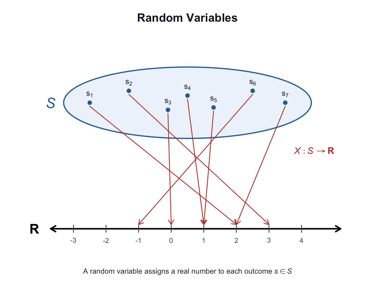
FIGURE 4.1: A random variable \(X\) is a function that maps each outcome in the sample space \(S\) to a real number.
A random variable is a deterministic function evaluated at a random outcome. The function \(X\) is deterministic; the randomness arises from the random outcome \(s\) to which it is applied.
Formally, a random variable is a measurable function. This condition ensures that probabilities such as \(\Pr(X\le x)\) are well-defined. In this book, all random variables considered satisfy this condition.
Many random variables take only integer values, such as the number of heads in three coin tosses; these are called discrete random variables. Many random variables take values in an interval, such as the height of a randomly chosen person; these are continuous random variables. Mixed random variables have both discrete probability mass and a continuous density component. In all cases, \(X(s)\) is a real number, but the set of possible values of \(X\) may be a finite set, a countable set (like the integers), or an interval in \(\mathbb{R}\).
Random variables are different from variables used in algebra. In algebra, a variable typically represents an unknown but fixed quantity. In contrast, a random variable represents a quantity whose value depends on the outcome of a random process.
Definition 4.2 (Domain, range and support) The domain of \(X\) is the sample space \(S\), and the range (or value set) is the set of real values taken by \(X\), denoted \(\mathcal{R}_X = \{X(s) \mid s \in S\}\), where \(\mathcal{R}_X \subseteq \mathbb{R}\).
The support of \(X\) is the set of values that can occur with non-zero probability.
Since \(X\) is a function, each \(s\in S\) is assigned to exactly one value \(X(s)\); however, multiple values of \(s\in S\) may be assigned to the same value of \(X(s)\). The variable is random since its value depends upon the outcome of the random process.
Example 4.1 (Rolling a die twice) Consider rolling a fair die twice. The sample space \(S\) (i.e., the domain of \(X\)) contains the \(36\) elements shown in Table 3.3: \[ S = \{ (1, 1), (1, 2), (1, 3), \dots, (6, 5), (6, 6)\}. \] However, we may be interested in the random variable \(X\), the product of the two numbers rolled. The random variable \(X\) assigns each element \(s\) of \(S\) to exactly one real number (in this case, to exactly one integer): \[\begin{align*} (1, 1) &\mapsto 1;\\ (1, 2) &\mapsto 2;\\ (1, 3) &\mapsto 3;\\ \vdots &\qquad \vdots\\ (6, 5) &\mapsto 30;\\ (6, 6) &\mapsto 36. \end{align*}\] Each element of the sample space is mapped to exactly one value of \(X\). However, multiple elements of the sample space can be mapped to the same value of \(X\): \[\begin{align*} (3, 4) &\mapsto 12; \quad\text{and}\\ (4, 3) &\mapsto 12; \quad\text{and}\\ (6, 2) &\mapsto 12; \quad\text{and}\\ (2, 6) &\mapsto 12. \end{align*}\] Writing \(X = 12\) means ‘the product of the numbers on the two rolls is \(12\)’.
The domain of \(X\) is the sample space \(S\), consisting of all \(36\) ordered pairs. The range of \(X\) is the set of distinct products obtainable: \[ \mathcal{R}_X = \{1, 2, 3, 4, 5, 6, 8, 9, 10, 12, 15, 16, 18, 20, 24, 25, 30, 36\}. \] \(\mathcal{R}_X\) contains only \(18\) elements, fewer than \(|S| = 36\), since several pairs give the same product (as shown above for \(X = 12\)).
Since every pair in \(S\) occurs with positive probability (\(1/36\) each), every value in the range also has positive probability, so the support and the range are identical here.
Once a random variable has been defined, events can be defined in terms of the values of the random variable. Random variables provide a convenient way to express events numerically; rather than listing specific outcomes, events can be described using inequalities or equations involving the random variable.
Example 4.2 (Rolling a die twice: range) In Example 4.1, the range of the random variable \(X\) is \[ \mathcal{R}_X = \{1, 2, 3, 4, 5, 6, 8, 9, 10, 12, 15, 16, 18, 20, 24, 25, 30, 36\}. \] The domain is the sample space, the set of all ordered pairs \[\begin{align*} S &= \{ (1, 1), (1, 2), (1, 3), \dots (3, 2), (3, 3), (3, 4),\dots (6, 5), (6, 6)\}\\ &= \{(r_1, r_2): r_1, r_2\in\{1, \dots, 6\}\}. \end{align*}\]
Example 4.3 (Rolling a die twice: events) The random variable \(X\) in Example 4.1 can be used to define different events. For example, Event \(A_1\) could be defined as \[ \{s \in S \mid X(s) > 10\}, \] usually written more succinctly as \(X > 10\). The values of the random variable corresponding to this event are \[ X = 11, 12. \] Other events can be defined also; for example: \[\begin{align*} A_2 &= \{ s \in S \mid 4 \le X(s) < 10 \} \quad\text{corresponding to}\quad X = 4, 5, 6, 7, 8, 9;\\ A_3 &= \{s \in S\mid X(s) < 0\} = \varnothing \quad\text{so there are no corresponding values of $X$};\\ A_4 &= \{s\in S\mid X(s) \text{ is prime}\} \quad\text{corresponding to}\quad X = 2, 3, 5. \end{align*}\]
Example 4.4 (Sum of two die rolls) Consider observing the rolls of two dice. The sample space contains \(36\) elements (Example 3.14), and can be denoted using the ordered pairs \((r_1, r_2)\), where \(r_1\) and \(r_2\) are the results of die \(1\) and \(2\) respectively. The sample space (the domain of \(X\)) is listed in Table 3.3. For example, \(s_1\) could be defined as the sample point \((1, 1)\).
The random variable \(Y\) can be defined on this sample space as: \[ Y(s) = \text{the sum of the two rolls in $s$} = r_1 + r_2. \] This definition assigns a real number to each outcome in the sample space:
| Sample space elements | Value of random variable \(Y\) |
|---|---|
| (1, 1) | 2 |
| (1, 2), (2, 1) | 3 |
| (1, 3), (2, 2), (3, 1) | 4 |
| \(\vdots\) | \(\vdots\) |
| (6, 6) | 12 |
For example, the elements of \(S\) assigned to \(Y = 4\) are \((1, 3)\), \((2, 2)\) and \((3, 1)\). Notice that many elements of the sample space can be assigned to the same value of the random variable (which is typical for random variables).
The domain of \(Y\) is the sample space \(S\); the range is \[ \mathcal{R}_Y = \{ Y(s) \mid s\in S\} = \{2, 3, \dots, 12\}. \]
Example 4.5 (Tossing a coin till a head appears) Consider the random process ‘tossing a coin until a Head is observed’. The sample space is \[ \Omega = \{H, TH, TTH, TTTH, \dots \}. \] The random variable \(N\) could be defined as ‘the number of tosses until the first head is observed’. \(\Omega\) is countably infinite. Each element of the sample space is assigned to a positive integer: \[\begin{align*} H\quad &\text{is assigned to $N = 1$};\\ TH\quad &\text{is assigned to $N = 2$};\\ TTH\quad &\text{is assigned to $N = 3$} \end{align*}\] and so on. Writing \(N = 2\) means ‘the number of tosses to observe the first head is two’.
Example 4.6 (Drawing two cards) Consider drawing two cards from a standard, well-shuffled pack of cards, and observing the colour of the card (B: Black; R: Red). The sample space \(\Omega\) is: \[ \Omega = \{ BB, BR, RR, RB\}, \] where the order represents the order in which the cards are drawn. Many random variables could be defined on this sample space; for example: \[\begin{align*} T&: \text{The number of black cards drawn};\\ M&: \text{The number of red cards drawn};\\ D&: \text{The number of black cards drawn,}\\ &\qquad \text{minus the number of red cards drawn}. \end{align*}\] These all assign a real number to each element of \(\Omega\); consider random variable \(D\), for instance:
| Sample space elements | Value of \(D\) |
|---|---|
| \(BR\) and \(RB\) | \(D = 0\) |
| \(BB\) | \(D = 2\) |
| \(RR\) | \(D = -2\) |
The domain is \(\Omega\), and the range is \(\mathcal{R}_D = \{ D(s) \mid s\in \Omega\} = \{-2, 0, 2\}\).
4.2 Discrete, continuous and mixed random variables
As observed earlier, random variables can be discrete, continuous, or mixed. Each are discussed in the sections that follow.
4.2.1 Discrete random variables
The examples used so far in this chapter has been examples of discrete random variables.
Definition 4.3 (Discrete random variable) A discrete random variable takes values in a finite or countable infinite set. Its distribution is described using a probability mass function.
Example 4.7 (Discrete rvs) In Example 4.1, the range of \(X\) contains exactly \(18\) values.
In Example 4.4, exactly \(11\) values of the random variable \(Y\) are possible: \(2, 3, \dots 12\).
In Example 4.5, the random variable \(N\) takes a countably infinite number of possible values: \(1, 2, 3, \dots\)
In Example 4.6, the random variable \(D\) can take one of three possible values: \(-2\), \(0\) or \(2\).
These are all discrete random variables.
The definition refers to the values of random variable, not to the sample space. Examples of discrete random variables include:
- The number of children aged under \(18\) living in a household.
- The number of errors per month.
- The number of incidents of lung cancer at a hospital in the last \(28\) days.
- The number of cyclones per season.
- The number of wins by a football team.
- The number of kangaroos observed in a five-hectare transect.
4.2.2 Continuous random variables
For a continuous sample space, the random variable is usually the identity function \(Y(s) = s\). For example, in Example 2.19 the sample space that describes how far a cricket ball can be thrown is already defined on the positive reals. Hence, we can define the random variable as \(T(s) = s\), where \(s\) is the distance specified in the sample space.
Definition 4.4 (Continuous random variable) A continuous random variable can take values in a continuum (an uncountable set of values), and \(\Pr(X = x) = 0\) for all \(x\). Its distribution is described using a probability density function.
A continuous random variable is one that can take values on a continuous scale (such as all real numbers in an interval), rather than only distinct separate values. The value of a continuous random variable can never, in principle, be measured exactly, so in practice needs to be rounded.
Example 4.8 (Heights) Height \(H\) is often recorded to the nearest centimetre (e.g., \(179\,\text{cm}\)) for convenience and practicality. Better measuring instruments may be able to record height to one or more decimal places of a centimetre. The range is \(\mathcal{R}_H =(0, \infty)\), or \(\mathcal{R}_H = \{ h\in \mathbb{R}\mid h > 0\}\).
Even though your height may not change, the notion of a random variable means that height varies from one realisation of the random process to another; that is, from one person to the next.
Examples of continuous random variables include:
- The volume of waste water treated at a sewage plant per day.
- The weight of hearts in rats.
- The lengths of the wings of butterflies.
- The yield of barley from a large paddock.
- The amount of rainfall recorded each year.
- The time taken to perform a psychological test.
- The percentage cloud cover.
Example 4.9 (Continuous rv) Let \(X\) have the density function \[ f_X(x) = \begin{cases} \lambda \exp(-\lambda x) & \text{for $x\ge 0$}\\ 0 & \text{for $x < 0$} \end{cases} \] for some \(\lambda > 0\). Suppose the sample space is defined as \(S = \mathbb{R}\) (i.e., \(X\) is, in principle, a real-valued measurement that could take any real value).
Here, the domain is \(S = \mathbb{R}\) and the range is \(\mathcal{R}_X = \mathbb{R}\), since \(X(s) = s\) for every \(s\in S\). The support is \([0, \infty)\), since \(f_X(x) = 0\) for all \(x < 0\).
The density can also be written in terms of the support: \[ f_X(x) = \lambda \exp(-\lambda x) \qquad \text{for $x\ge 0$}. \]
4.2.3 Mixed random variables
Some random variables are not completely discrete or continuous; these are called mixed random variables. A common example in applications is a random variable that is continuous on the positive real numbers, with a discrete probability mass at zero.
Definition 4.5 (Mixed random variable) A mixed random variable has a distribution with both discrete probability mass and a continuous density component.
A mixed random variable has some values with positive probability and also a continuous range of possible values described by a density function. In this book, we only consider mixed random variables with a point mass at \(X = 0\) and a continuous component on \(\mathbb{R}_{+}\), although more general mixtures are possible.
Example 4.10 (Vehicle wait times) Consider the time spent by vehicles waiting at a set of traffic lights before proceeding through the intersection.
If the light is green on arrival, the wait time is zero: the vehicle proceeds immediately. Thus, there is a positive probability that the waiting time is exactly zero. If the light is red on arrival, the vehicle waits a continuously varying amount of time until the light turns green.
The waiting time is therefore a mixed random variable, with a discrete probability mass at zero and a continuous distribution for positive waiting times.
Examples of mixed random variables include:
- The amount of rainfall that falls in a month (zero, or a continuous amount).
- The weight of fruit produced per tree (zero if no fruit is produced, or a continuous amount).
- The mass of fish-catch per trawl (zero if no fish are caught, or a continuous amount).
- Insurance claim size (zero if no claim, or a continuous positive amount otherwise)
- Purchase amount in a store (zero if no purchase, positive continuous amount otherwise)
4.3 Probability functions
The previous section introduced random variables: real values assigned to outcomes in the sample space. Often, many elements of the sample space were assigned to the same value of the random variable. Therefore, probabilities can be assigned to various values of the random variable, to develop a probability model for the random variable.
A model describes theoretical patterns over infinite trials.
On any single roll of a die, a ![]() may or may not occur, but theoretically (and for infinite rolls) we expect a
may or may not occur, but theoretically (and for infinite rolls) we expect a ![]() to appear \(1/6\) of the time.
A probability model describes the probability that various values of the random variable might appear on any one realisation in theory.
to appear \(1/6\) of the time.
A probability model describes the probability that various values of the random variable might appear on any one realisation in theory.
This probability model is called the probability function.
Example 4.11 (Tossing coin outcomes) Consider tossing a coin twice and observing the outcome of the two tosses. Since a random variable is a real-valued function, simply observing the outcome as \(HT\), for example, does not define a random variable.
We could define the random variable of interest, say \(H\), as the number of heads on the two tosses of the coin. The sample space for the experiment is \[ S = \{ TT, TH, HT, HH\}. \] The connection between the sample space and \(H\) is shown in the table below. In this case, the range of \(H\) is \(\mathcal{R}_H = \{0, 1, 2\}\). The probability of observing each value of \(H\) can be computed using classical probability:
| Element of \(S\) | Function \(H(s)\) | Value of \(H\) | \(\Pr(s_i)\) |
|---|---|---|---|
| \(s_1 = TT\) | \(H(s_1)\): Number of heads in \(s_1\) | 0 | \(1/4\) |
| \(s_2 = TH\) | \(H(s_2)\): Number of heads in \(s_2\) | 1 | \(1/4\) |
| \(s_3 = HT\) | \(H(s_3)\): Number of heads in \(s_3\) | 1 | \(1/4\) |
| \(s_4 = HH\) | \(H(s_4)\): Number of heads in \(s_4\) | 2 | \(1/4\) |
The probability function could be defined as \[\begin{align*} \Pr(H = 0):&\quad 1/4\\ \Pr(H = 1):&\quad 1/2\\ \Pr(H = 2):&\quad 1/4\\ \Pr(H = h):&\quad 0\quad \text{for all other values of $h$}. \end{align*}\]
Probability functions are written and interpreted differently, depending on whether the random variable is a discrete, continuous or mixed random variable.
4.3.1 Discrete random variables: probability mass functions
For a discrete random variable, the probability function indicates how probabilities are assigned to the values of the discrete random variable. For a discrete random variable, the probability function is often called the probability mass function (or PMF).
Definition 4.6 (Discrete probability mass function) Let \(X\) be a discrete random variable with range \(\mathcal{R}_X\). The probability mass function (or PMF), denoted \(p_X(x)\), assigns a probability to each outcome \(x_i\) such that \(p_X(x_i) = \Pr(X = x_i)\). The domain of the probability function \(p_X(x)\) is the set of values that \(X\) can take.
This function must satisfy: \[\begin{align} p_X(x) &\geq 0 \quad \text{for all } x \in \mathcal{R}_X \notag\\ \sum_{x_i \in \mathcal{R}_X} p_X(x_i) &= 1. \end{align}\] The collection of all pairs \(\{(x_i, p_X(x_i))\}\) for all \(i\) constitutes the probability distribution of \(X\).
Probability functions usually depend on values that determine the shape, location, scale, or some other feature of the function. These values are called parameters.
Definition 4.7 (Parameter) A parameter is a fixed numerical characteristic of a probability distribution. Parameters are typically unknown and fixed.
When a PMF depends on one or more parameters \(theta\), this is made explicit by writing \(p_X(x; \theta)\) for one parameter or \(p_X(x; \theta_1, \theta_2, \dots)\) for multiple parameters, where the semicolon separates the variable \(x\) from the parameters. For example, a PMF for a random variable \(X\) depending on parameters \(\alpha\) and \(\beta\) would be written \(p_X(x; \alpha, \beta)\).
The following properties of the probability function are implied by the definition and the rules of probability.
- \(p_X(t) \ge 0\) for all values of \(t\); that is, probabilities are never negative.
- \(\displaystyle \sum_{t \in \mathcal{R}_X} p_X(t) = 1\) where \(\mathcal{R}_X\) is the range of \(X\); that is, the probability function covers the probability over all possible sample points in the sample space.
- \(p_X(t) = 0\) if \(t \notin \mathcal{R}_X\).
- For an event \(A\subseteq\mathcal{R}_X\) defined on a sample space \(S\), the probability of event \(A\) is \[ \Pr(A) = \sum_{t\in A} p_X(t). \]
The probability distribution of a discrete random variable \(X\) can be represented by listing each outcome with its probability; giving a formula; using a table; or using a graph which displays the probabilities \(p(x)\) corresponding to each \(x\in \mathcal{R}_X\).
Sometimes the probability function is denoted \(p(x)\) rather than \(p_X(x)\). Using the subscript avoids confusion in situations where many random variables are considered at once. The subscript is used throughout this book.
The probability distribution of a random variable is a description of the range of the variable and the associated assignment of probabilities.
Example 4.12 (The larger of two numbers) Five balls numbered \(1\), \(2\), \(3\), \(4\) and \(5\) are in an urn. Two balls are selected at random without replacement. Consider finding the probability distribution of the larger of the two numbers. When finding the larger of two numbers, the order is not important, so combinations are appropriate, and the number of possible outcomes is therefore \[ \binom{5}{2} = 10. \] These are easily listed: the sample space is: \[ S =\{ (1, 2), (1, 3), (1, 4), (1, 5), (2, 3), (2, 4), (2, 5), (3, 4), (3, 5), (4, 5)\}, \] where all \(10\) elements are equally likely. Then, let \(X\) be the random variable ‘the larger of the two numbers chosen’, so that \(\mathcal{R}_X = \{2, 3, 4, 5\}\). Listing the probabilities: \[\begin{alignat*}{3} \Pr(X = 2) &= \Pr\big((1, 2)\big) &\quad &= 1/10;\\ \Pr(X = 3) &= \Pr\big((1, 3) \text{ or } (2, 3)\big) &\quad &= 2/10;\\ \Pr(X = 4) &= \Pr\big((1, 4) \text{ or } (2, 4) \text{ or } (3, 4)\big) &\quad &= 3/10;\\ \Pr(X = 5) &= \Pr\big((1, 5) \text{ or } (2, 5) \text{ or } (3, 5)\text{ or } (4, 5)\big) &\quad &= 4/10;\\ \Pr(\text{other values of } X) & \text{ } &\quad &= 0. \end{alignat*}\] This is the probability distribution of \(X\), which could also be given in a table (Table 4.1), a graph (Fig. 4.2), or as a formula: \[ \Pr(X = x) = (x - 1)/10\qquad\text{for $x = 2, 3, 4, 5$}. \] The probability is zero for all values not in \(\mathcal{R}_X\).
| \(x\) | 2 | 3 | 4 | 5 |
| Probability | 0.1 | 0.2 | 0.3 | 0.4 |
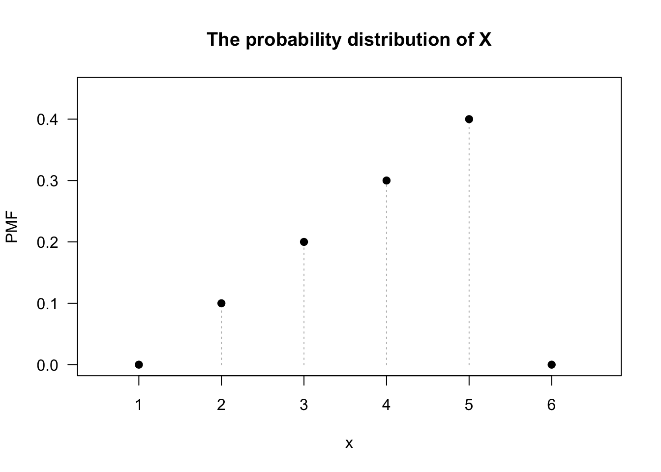
FIGURE 4.2: The probability function for the larger of two numbers drawn.
Show R code
plot( x = 1:6,                           # The values for which PMF > 0
      y = c(0, 0.1, 0.2, 0.3, 0.4, 0),   # The values of f(y)
      xlim = c(0.5, 6.6), ylim = c(0, 0.45),
      type = "h",             # type = "h": vertical lines
      lty = 3,                # lty = 3: Dotted lines
      las = 1,                # las = 1: Axis labels horizontal
      col = "grey",           # Use the colour grey
      main = "The probability distribution of X",
      xlab = "x",             # Label for horizontal axis
      ylab = "PMF"            # Label for vertical axis
)
points( x = 1:6,  ### Adds the points on top of the vertical lines
        y = c(0, 0.1, 0.2, 0.3, 0.4, 0),
        pch = 19)
Example 4.13 (Parameters in a PMF) Define a random variable \(X\), with probability mass function \[ p_X(x; a) = \begin{cases} ax & \text{for $x = 1, 2$};\\ 1 - 3a & \text{for $x = 3$} \end{cases} \] for \(0 < a < (1/3)\). The PMF has a parameter \(a\). For example, if \(a = 0.1\), then \[ p_X(x; a = 0.1) = \begin{cases} 0.1x & \text{for $x = 1, 2$};\\ 0.7 & \text{for $x = 3$}. \end{cases} \]
Example 4.14 (Tossing heads) Suppose a fair coin is tossed twice and the uppermost face is noted, as in Example 4.11. The probability function is \[ p_H(h) = \Pr(H = h) = \begin{cases} 0.25 & \text{if $h = 0$};\\ 0.5 & \text{if $h = 1$};\\ 0.25 & \text{if $h = 2$}. \end{cases} \] More succinctly, \[\begin{align*} p_H(h) &= \Pr(H = h) \\ &= (0.5)\,0.5^{|h - 1|} \qquad \text{for $h = 0$, $1$ or $2$}. \end{align*}\] This information can also be presented as a table (Table 4.2) or graph (Fig. 4.3). Note that \(\sum_{t \in \{0, 1, 2\}} p_H(t) = 1\) and \(p_H(h)\ge0\) for all \(h\), as required of a probability function.
| \(h\) | 0 | 1 | 2 |
| \(\Pr(H = h)\) | 0.25 | 0.5 | 0.25 |
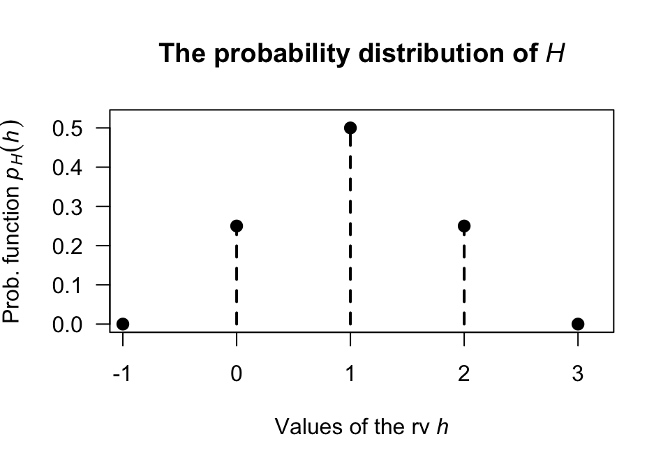
FIGURE 4.3: The probability function for \(H\), the number of heads on two tosses of a coin.
4.3.2 Continuous random variables: probability density functions
In the discrete case, probability can be distributed over distinct points (possibly a countably infinite number) where each point has non-zero mass. However, in the continuous case, mass cannot be thought of as an attribute of a point but rather of a region surrounding a point. The ideas from Sect. 3.7 are relevant here.
Definition 4.8 (Continuous probability density function) The probability density function (or PDF) of a continuous random variable \(X\) is a function \(f_X(x)\) such that:
- \(f_X(x) \geq 0\) for all \(x \in \mathcal{R}_X\); and
- The total area under the curve is \(1\): \[ \int_{\mathcal{R}_X} f_X(x) \, dx = 1. \]
The domain of the probability function \(f_X(x)\) is the set of values that \(X\) can take.
The probability that \(X\) falls within a specific region \(A\) is the area under the curve: \[ \Pr(X \in A) = \int_A f_X(x) \, dx. \]
As with PMFs, when a PDF depends on one or more parameters \(\theta\), this is made explicit by writing \(f_X(x; \theta)\) for one parameter or \(f_X(x; \theta_1, \theta_2, \dots)\) for multiple parameters, where the semicolon separates the variable \(x\) from the parameters.
We are usually only concerned with \((a, b)\in \mathcal{R}_X\), but it makes sense to think of the PDF as defined for all \(x\), insisting that \(f_X(x) = 0\) for \(x\notin \mathcal{R}_X\). This definition implies that areas under the graph of the PDF represent probabilities and leads to the following properties:
- \(f_X(x) \ge 0\) for all \(-\infty < x < \infty\): the density function is never negative.
- \(\displaystyle \int_{-\infty}^\infty f_X(x)\,dx = 1\): the total probability is one.
- For an event \(A\subseteq \mathcal{R}_X\) defined on a sample space \(S\), the probability of event \(A\) is \[ \Pr(A) = \int_{A} f_X(x)\, dx. \]
- Since exact values are not possible: \[\begin{align*} & \Pr(a < X \le b) = \Pr(a < X < b)\\ {}={} & \Pr(a \le X < b) = \Pr(a \le X \le b) = \int_a^b f_X(x)\,dx \end{align*}\]
Properties 1 and 2 are sufficient to prove that a function is a probability density function That is, to show that some function \(g(x)\) is a PDF, showing that \(g(x) \ge 0\) for all \(-\infty < x < \infty\) and that \(\int_{-\infty}^\infty g(x)\,dx = 1\) is sufficient.
Property 4 results from noting that if \(X\) is a continuous random variable, \(\Pr(X = a) = 0\) for any and every value \(a\) for the same reason that a point has mass zero.
The value of a probability density function at some point \(x\) does not represent a probability, but rather a probability density. Hence, the probability density function can have any non-negative value of arbitrary size at a specific value of \(X\).
Example 4.15 (Probability density function) Consider the continuous random variable \(W\) with the probability density function \[ f_W(w) = 2w\qquad\text{for $0 < w < 1$} \] where \(\mathcal{R}_X = (0, 1)\). The probability is zero for values of \(x\) outside \(\mathcal{R}_X\).
The probability \(\Pr(0 < W < 0.5)\) can be computed in one of two ways. One is to use calculus: \[ \Pr(0 < W < 0.5) = \left[w^2\right]_0^{0.5} = 0.25. \] Alternately, the probability can be computed geometrically from the graph of the PDF (Fig. 4.4). The region corresponding to \(\Pr(0 < W < 0.5)\) is triangular; integration simply finds the area of this triangle. Thus, the area can be found using the area of a triangle directly: the length of the base of the triangle, times the height of the rectangle, divided by two: \[ 0.5 \times 1 /2 = 0.25, \] and the answer is the same as before.
Note that \(f_W(w)\) is greater than one for some values of \(w\). Since \(f_W(w)\) does not represent probabilities at each point (as \(W\) is continuous), this is not problematic. However, \(\int_{\mathbb{R}} f_W(w) \, dw = 1\) as required of a probability density.
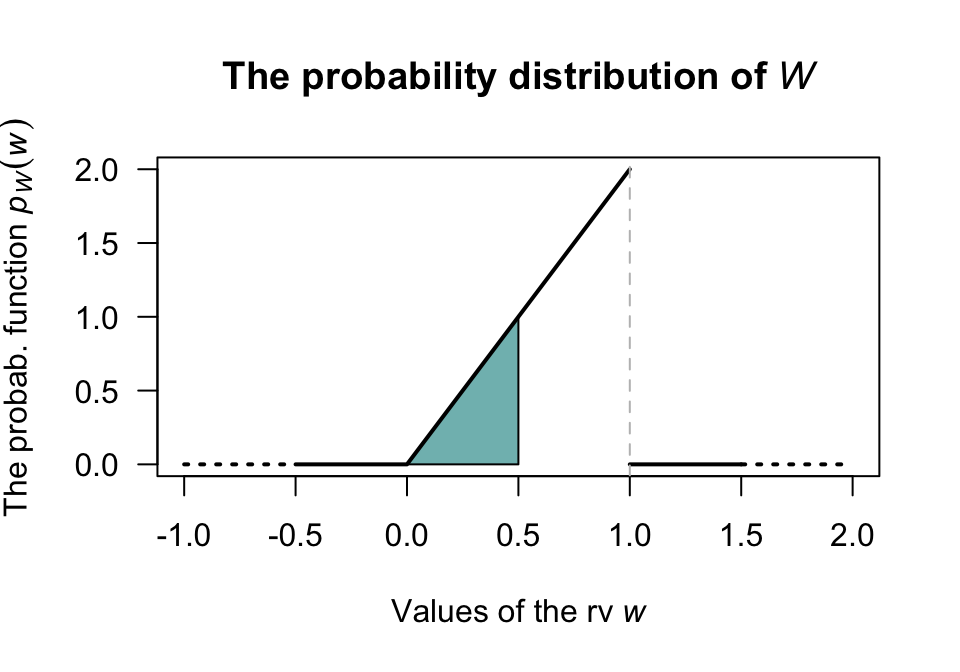
FIGURE 4.4: The probability function for \(W\). The shaded area represents \(0 < W < 0.5\).
Example 4.16 (Probability density function) A random variable \(T\) has the probability density function \[ f_T(t; \alpha) = \begin{cases} t/\alpha^2 & \text{for $0 < t \le \alpha$};\\ (2\alpha - t)/\alpha^2 & \text{for $\alpha < t < 2\alpha$} \end{cases} \] for \(\alpha > 0\) (Fig. 4.5). Here, \(\alpha\) is a parameter. Note that \(\int_0^{2\alpha} f_T(t)\,dt = 1\) for all values of \(\alpha\).
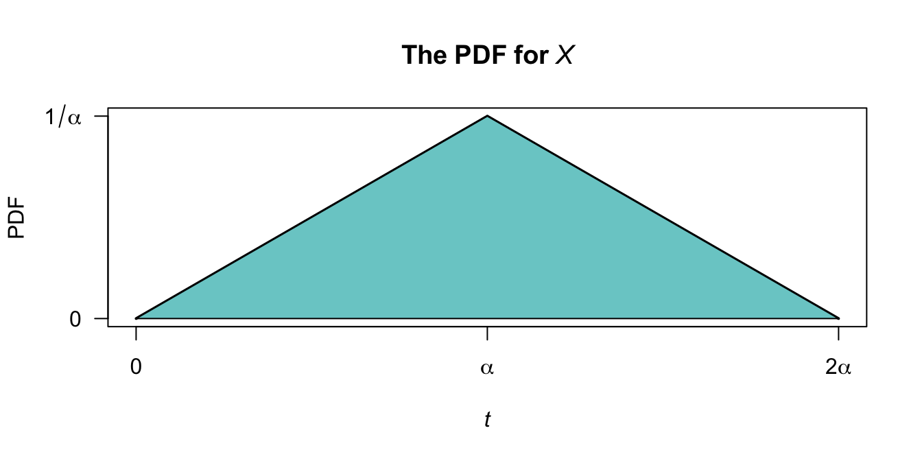
FIGURE 4.5: The PDF for the random variable \(T\) with parameter \(\alpha\).
4.3.3 Mixed random variables
Some random variables are not entirely continuous nor entirely discrete, but have components of both. These random variables are called mixed random variables.
Definition 4.9 (Mixed probability function) The probability function of a mixed random variable \(X\) is characterized by:
- A probability mass function \(p_X(x)\) at each discrete mass point \(x_i \in \mathcal{R}_X^d\), where \(\mathcal{R}_X^d \subseteq \mathcal{R}_X\) is the discrete part of the range, and
- A probability density function \(f_X(x)\) over the continuous part \(\mathcal{R}_X^c \subseteq \mathcal{R}_X\).
These must satisfy:
- \(p_X(x_i) \geq 0\) for all \(x_i \in \mathcal{R}_X^d\) and \(f_X(x) \geq 0\) for all \(x \in \mathcal{R}_X^c\), and
- The total probability is \(1\): \[ \sum_{x_i \in \mathcal{R}_X^d} p_X(x_i) + \int_{\mathcal{R}_X^c} f_X(x)\,dx = 1. \]
Again, if the mass function or the density function depends on one or more parameters, this is made explicit by writing \(p_X(x; \theta, \dots)\) or \(f_X(x; \theta, \dots)\) as appropriate, where the semicolon separates the variable \(x\) from the parameters.
The probability that \(X\) falls within a region \(A\) is: \[ \Pr(X \in A) = \sum_{x_i \in A \cap \mathcal{R}_X^d} p_X(x_i) + \int_{A \cap \mathcal{R}_X^c} f_X(x)\,dx. \]
The most common example of a mixed random variable is when an exact probability exists when the value of the random variable is zero (discrete), and the random variable is then continuous for positive values. In other words, when \(\mathcal{R}_X^d = \{0\}\) and \(\mathcal{R}_X^c = (0, \infty)\).
Example 4.17 (Mixed random variable) In a factory producing diodes, a proportion \(p\) of the diodes fail immediately. The distribution of the lifetime (in hundreds of days), say \(Y\), of the diodes is given by a discrete component at \(y = 0\) for which \(\Pr(Y = 0) = p\), and a continuous part for \(y > 0\) with density \[ f_Y(y; p) = (1 - p) \exp(-y) \quad \text{if $y > 0$.} \] Here, \(f_Y(y)\) is not itself a PDF over \(\mathbb{R}\), as it doesn’t integrate to one; however the total probability is \[ p + \int_0^\infty (1 - p)\exp(-y) \, dy = p + (1 - p) = 1 \] as required.
Consider a diode for which \(p = 0.4\). The distribution is displayed in Fig. 4.6 where a solid dot is included to show the discrete mass at \(Y = 0\).
Representing the probability distribution in this mixed case is difficult, because of the need to combine a probability density function and a probability mass function. These difficulties are overcome by using the distribution function (Sect. 4.4).
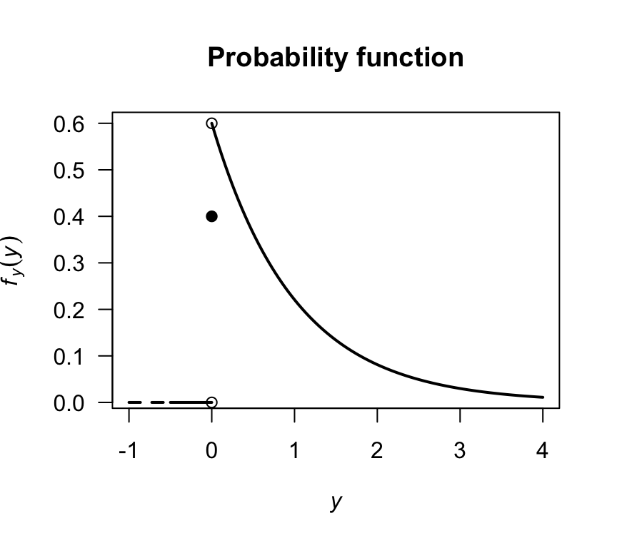
FIGURE 4.6: The probability function for the diodes example.
4.4 Distribution functions
4.4.1 General ideas
Another way of describing random variables is using a distribution function (DF), also called a cumulative distribution function (CDF). The DF gives the probability that a random variable \(X\) is less than or equal to a given value of \(x\).
Definition 4.10 (Distribution function) For any random variable \(X\) the distribution function, \(F_X(x; \theta_1, \dots)\) with parameters \(\theta_1, \dots\), is \[ F_X(x; \theta_1, \dots) = \Pr(X \leq x) \quad \text{for $x\in\mathbb{R}$}. \]
The distribution function applies to discrete, continuous or mixed random variables. Importantly, the distribution functions is defined for all real numbers.
If \(X\) is a discrete random variable with range \(\mathcal{R}_X\), then the DF is \[\begin{align*} F_X(x) &= \Pr(X \leq x)\\ &= \sum_{x_i \leq x} \Pr(X = x_i)\text{ for }x_i\in \mathcal{R}_X,\text{ and }-\infty < x < \infty. \end{align*}\] If \(X\) is a continuous random variable, the DF is \[\begin{align*} F_X(x) &= \Pr(X \leq x)\\ &= \int^x_{-\infty} f(t)\,dt \text{ for } -\infty < x < \infty. \end{align*}\]
Properties of the distribution function include:
- \(0\leq F_X(x)\leq 1\) because \(F_X(x)\) is a probability.
- \(F_X(x)\) is a non-decreasing function of \(x\). That is, if \(x_1 < x_2\) then \(F_X(x_1) \leq F_X(x_2)\).
- \(\displaystyle{\lim_{x\to \infty} F_X(x)} = 1\) and \(\displaystyle{\lim_{x\to -\infty} F_X(x)} = 0\).
- \(\Pr(a < X \leq b) = F_X(b) - F_X(a)\).
- If \(X\) is discrete, then \(F_X(x)\) is a step-function. If \(X\) is continuous, then \(F_X\) will be a continuous function for all \(x\).
4.4.2 Discrete random variables
The above ideas can be applied in the discrete case, but care is needed at the values of the random variable where the probability is non-zero.
Example 4.18 (Tossing heads) Consider the simple example in Example 4.14 where a coin is tossed once. The probability function for \(H\) is given in that example in numerous forms. To determine the distribution function, first note that when \(h < 0\), the accumulated probability is zero; hence, \(F_H(h) = 0\) when \(h < 0\). At \(h = 0\), the probability of \(0.25\) is accumulated all at once, and no more probability is accumulated until \(h = 1\). Thus, \(F_H(h) = 0.25\) for \(0 \le h < 1\). Continuing, the distribution function is \[ F_H(h) = \begin{cases} 0 & \text{for $h < 0$};\\ 0.25 & \text{for $0\le h < 1$};\\ 0.75 & \text{for $1\le h < 2$};\\ 1 & \text{for $h\ge 2$}. \end{cases} \] The distribution function can be displayed graphically, being careful to clarify what happens at \(H = 1\), \(H = 2\) and \(H = 3\) using open or filled circles (Fig. 4.7).
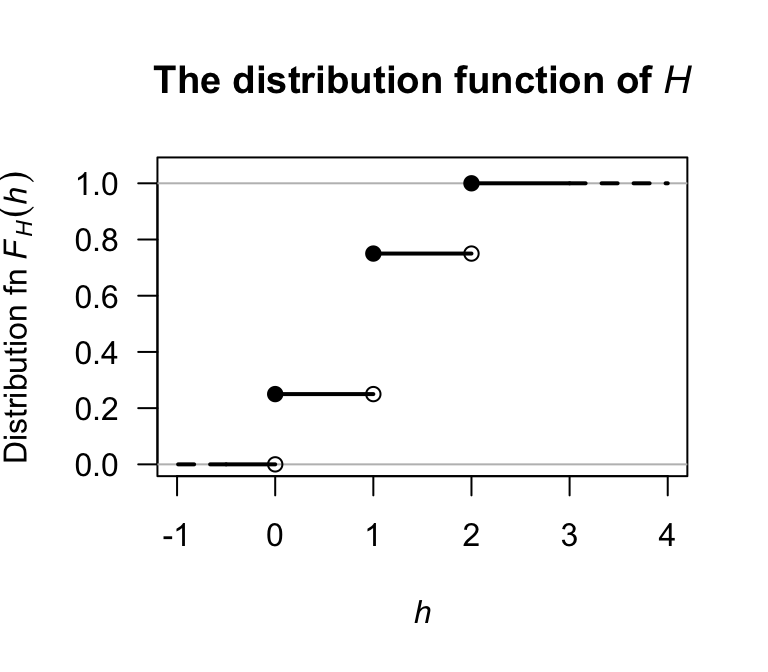
FIGURE 4.7: A graphical representation of the distribution function for the tossing-heads example. The filled circles contain the given point, while the empty circles omit the given point.
4.4.3 Continuous random variables
The same ideas apply for continuous random variables, but probabilities are accumulated using integrations rather than summations.
Example 4.19 (Distribution function) Consider a continuous random variable \(V\) with PDF \[ f_V(v) = v/2\qquad\text{for $0 < v < 2$}. \] The distribution function is zero whenever \(v\le 0\). For \(0 < v < 2\), \[ F_V(v) = \int_0^v t/2\,dt = v^2/4. \] Whenever \(v\ge 2\), the DF is one. So the DF is \[ F_V(v) = \begin{cases} 0 & \text{if $v\le 0$};\\ v^2/4 & \text{if $0 < v < 2$};\\ 1 & \text{if $v\ge 2$.} \end{cases} \] A picture of the distribution function is shown in Fig. 4.8.
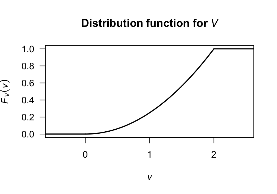
FIGURE 4.8: The distribution function for \(V\).
For the integral, do not write \[ \int_0^v v/2\,dv. \] Having the variable of integration as a limit on the integral and also in the function to be integrated makes no sense. Either write the integral as given in the example, or write \(\int_0^t v/2\,dv = t^2/4\) and then change the variable from \(t\) to \(v\).
4.4.4 Mixed random variables
The distribution function for mixed random variables follow the same ideas as above, using summations and integrations as appropriate.
Example 4.20 (Mixed random variable) Example 4.17 discussed the mixed random variable \(Y\), the lifetimes of diodes (in hundreds of days). A proportion of the diodes \(p = 0.4\) fail immediately (i.e., \(\Pr(Y = 0) = 0.4\)). For other diodes, the distribution function of \(Y\) is described by \[\begin{align*} F_Y(y; p) &= \Pr(Y\le y)\\ &= p + \int_0^y f_Y(t)\, dt \\ &= p + (1 - p) \int_0^y\exp(-t)\, dt \\ &= p + (1 - p) [1 - \exp(-y)]\\ &= 0.4 + 0.6 [1 - \exp(-y)] \end{align*}\] for \(y > 0\). The probability distribution is displayed in Fig. 4.9 where a solid dot is included to show the discrete part.
The complete distribution function, when \(p = 0.4\), is: \[ F_Y(y) = \begin{cases} 0 & \text{if $y < 0$}\\ 0.4 & \text{if $y = 0$}\\ 0.4 + 0.6(1 - \exp(-y)) & \text{if $y > 0$}. \end{cases} \] The total probability is \[ 0.4 + 0.6\int_0^\infty \exp(-y) \, dy = 1 \] as required. In addition, as required, \[ \lim_{y \to\infty} F_Y(y) = 0.4 + 0.6 = 1. \]
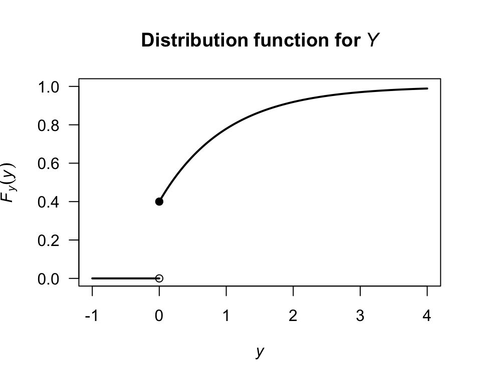
FIGURE 4.9: The distribution function for the diodes example.
4.4.5 Recovering the PF from the DF
We have seen how to find \(F_X(x)\) given \(\Pr(X = x)\), or to find \(F_X(x)\) given \(f_X(x)\). But can we proceed in the other direction too? That is, given \(F_X(x)\), how do we find the corresponding probability function?
As seen from the graph of the distribution in Example 4.18, the values of \(x\) where a ‘jump’ in \(F_X(x)\) occurs are the points in the range with positive probabilities, and the probability associated with a particular point in \(\mathcal{R}_X\) is the ‘height’ of the corresponding jump. This implies \[\begin{equation} p_X(x_j) = \Pr(X = x_j) = F_X(x_j) - F_X(x_{j - 1}). \tag{4.1} \end{equation}\]
Example 4.21 (Mass function from distribution function) Consider the DF for a discrete random variable \(X\): \[ F_X(x) = \begin{cases} 0 & \text{for $x < 10$;}\\ 0.1 & \text{for $10 \le x < 11$;}\\ 0.4 & \text{for $11 \le x < 15$;}\\ 0.9 & \text{for $15 \le x < 17$;}\\ 1 & \text{for $x \ge 17$.} \end{cases} \] To find the PMF, use Eq. (4.1): \[ f_X(x) = \begin{cases} 0.1 & \text{for $x = 10$}\\ 0.3 & \text{for $x = 11$}\\ 0.5 & \text{for $x = 15$}\\ 0.1 & \text{for $x = 17$} \end{cases} \] As shown in Fig. 4.10, the discrete jumps in the DF correspond to the value of the PMF at those values of \(X\).
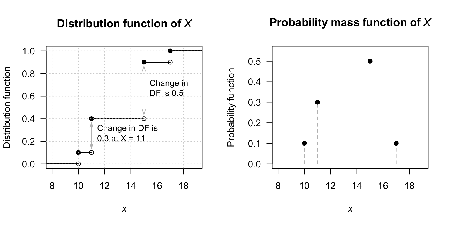
FIGURE 4.10: Left: the distribution function of \(X\). Right: the probability mass function of \(X\).
When \(X\) is continuous, from the Fundamental Theorem of Calculus, \[\begin{equation} f_X(x) = \frac{d}{dx} F_X(x) \quad \text{where the derivative exists.} \tag{4.2} \end{equation}\]
Example 4.22 (Density function from distribution function) Consider the DF for a continuous random variable \(X\): \[ F_X(x) = \begin{cases} 0 & \text{for $x < 0 $;}\\ x(2 - x) & \text{for $0 \le x \le 1$;}\\ 1 & \text{for $x > 1$.} \end{cases} \] To find the PDF, use Eq. (4.2): \[\begin{align*} f_X(x) &= \begin{cases} \displaystyle\frac{d}{dx} 0 & \text{for $x < 0 $;}\\[6pt] \displaystyle\frac{d}{dx} x(2 - x) & \text{for $0 \le x \le 1$;}\\[6pt] \displaystyle\frac{d}{dx} 1 & \text{for $x > 1$} \end{cases} \\ &= \begin{cases} 0 & \text{for $x < 0 $;}\\ 2(1 - x) & \text{for $0 \le x \le 1$;}\\ 0 & \text{for $x > 1$} \end{cases} \end{align*}\] which is usually written as \(f_X(x) = 2(1 - x)\) for \(0 < x < 1\).
4.5 Survival functions
In many applications (suc as medical research, climatology, engineering, and insurance), the probability remaining beyond a certain values is of more interest than the probability that an event has already occurred (i.e., the distribution function). This is akin to observing the probability that the quantity ‘survives’ beyond a given value.
The survival function, denoted \(S_X(x)\) and sometimes called the reliability function, is defined as the probability that the random variable \(X\) exceeds a value \(x\): \[\begin{equation} S_X(x; \theta_1, \dots) = \Pr(X > x) \tag{4.3} \end{equation}\] for parameters \(\theta_1, \dots\). Since \(F_X(x) = \Pr(X \le x)\), the survival function is simply the complement of the distribution function: \[ S_X(x; \theta_1, \dots) = 1 - F_X(x; \theta_1, \dots). \]
Properties of the survival function include:
- \(0\leq S_X(x)\leq 1\) because \(S_X(x)\) is a probability.
- \(S_X(x)\) is a non-increasing function of \(x\). That is, if \(x_1 < x_2\) then \(S_X(x_1) \geq S_X(x_2)\).
- \(\displaystyle{\lim_{x\to \infty} S_X(x)} = 0\) and \(\displaystyle{\lim_{x\to -\infty} S_X(x)} = 1\).
- \(\Pr(a < X \leq b) = S_X(a) - S_X(b)\).
- If \(X\) is discrete, then \(S_X(x)\) is a step-function. If \(X\) is continuous, then \(S_X\) will be a continuous function for all \(x\).
- The point where \(F_X(x) = S_X(x) = 0.5\) is the median of the distribution.
For continuous variables, \(\Pr(X > x) = \Pr(X \ge x)\). For discrete variables, \(S_X(x)\) is the probability of the event occurring at any step strictly greater than \(x\).
Example 4.23 (Survival function) Suppose the time \(X\) (in years) until a specific LED bulb fails has a probability density function \[ f_X(x) - \exp(-x/2) \quad\text{for $x > 0$}. \] The distribution function is \(F_X(x) = 1 - \exp(-x/2)\), so the survival function is (Fig. 4.11) \[ S_X(x) = 1 - \left[1 - \exp(-x/2)\right] = \exp(-x/2). \] At \(x = 0\), the bulb has just been turned on, and \(F_X(0) = 0\) (probability of failing instantly is zero) and \(S_X(0) = 1\) (\(100\)% chance the bulb has survived to the start). As \(x \to \infty\), \(F_X(x)\) approaches \(1\), while \(S_X(x)\) approaches \(0\): eventually, every bulb ‘dies’.
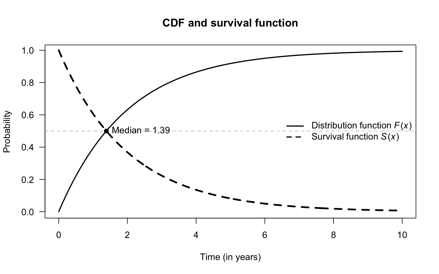
FIGURE 4.11: Relationship between distribution and survival functions
In the discrete case, the definition of the survival function requires precision regarding the boundaries.
Example 4.24 (Survivor function) Suppose a fair six-sided die is rolled.
Let \(X\) be the number of rolls until the first ![]() .
The probability mass function is
\[
p_X(x) = (1/6)^x\quad\text{for x = $1, 2, 3, 4, \dots$}.
\]
The distribution function gives the probability of taking fewer than or equal to \(x\) rolls to obtain a
.
The probability mass function is
\[
p_X(x) = (1/6)^x\quad\text{for x = $1, 2, 3, 4, \dots$}.
\]
The distribution function gives the probability of taking fewer than or equal to \(x\) rolls to obtain a ![]() .
The survival function \(S_X(x)\) gives the probability that it takes more than \(x\) rolls to roll a
.
The survival function \(S_X(x)\) gives the probability that it takes more than \(x\) rolls to roll a ![]() .
.
The DF is defined such that \(F_X(x) = \Pr(X \le x)\), and so includes the probability that \(X\) is exactly \(x\). However, the survival function, defined as \(S_X(x) = \Pr(X > x)\), excludes the probability that \(X\) is exactly the value \(x\). Since \(S_X(x)\) excludes the point \(x\), at the ‘jump’ points (like \(x = 1\) rolls), the survival probability \(S_X(1)\) is the probability that \(2\) or more rolls are needed. The distribution and survival functions are compared in Fig. 4.12.
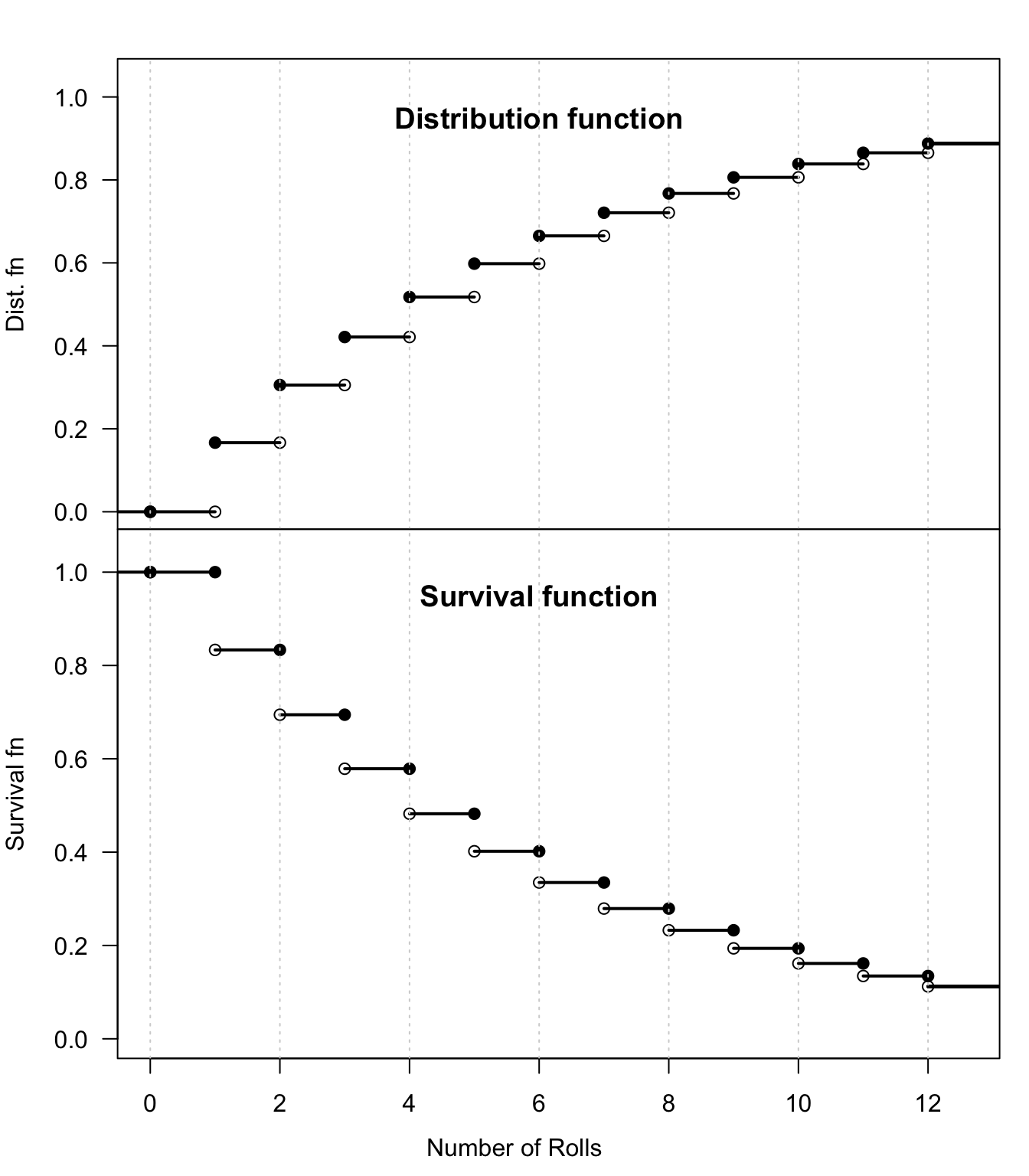
FIGURE 4.12: Relationship between distribution and survival functions
4.6 Quantile functions
For a random variable \(X\), the distribution function \(F_X(x)\) computes the probability that \(X < x\) for some given value of \(x\). The value of \(F_X(x)\) is a probability, so is a value between \(0\) and \(1\).
The quantile function \(Q_X(p)\) is the inverse of the distribution function; it takes a value between \(0\) and \(1\) (denoted \(p\)), and returns the smallest value \(x\) such that \(F_X(x) \ge p\) for given values of \(p\). The \(p\)-quantile of a distribution is a value \(x\) such that a fraction \(p\) of the distribution lies at or below \(x\). For example, the \(0.9\)-quantile (or the \(90\)% quantile) is the smallest value with (at least) \(90\)% of the distribution below or at the value. The median is the \(0.5\)-quantile—half the distribution (i.e., \(50\)%) is on each side of the median.
More formally, \[\begin{equation} Q_X(p; \theta_1, \dots) = \inf\{x \in \mathbb{R} \mid F_X(x; \theta_1, \dots) \ge p\}\quad\text{for $0 < p < 1$} \tag{4.4} \end{equation}\] where ‘inf’ is the ‘infimum’, the greatest lower bound of the set, and \(\theta_1, \dots\) are the parameters. In practice this refers to the leftmost value \(x\) where the distribution function \(F_X(x)\) reaches or exceeds a target probability \(p\).
When \(X\) is a continuous random variable and \(F_X(x)\) is a strictly increasing function, the quantile function is the inverse of the distribution function, and we can write \[ Q_X(p; \theta_1, \dots) = F_X^{-1}(p; \theta_1, \dots). \]
At the endpoints (\(p = 0\) and \(p = 1\)), some ambiguity exists. Some authors set \(Q_X(0) = \min\{x \mid F_X(x) > 0\}\), which is the smallest support point with a positive mass. Other authors define \(Q_X(0) = \lim_{p\downarrow 0} Q_X(p)\), which for some distributions may lead to \(Q_X(0) \to -\infty\).
Similarly, some authors leave \(Q_X(1)\) undefined. Others define it as the smallest value \(x\) where the distribution function first reaches 1, i.e., \(Q_X(1) = \inf\{x \mid F_X(x) = 1\}\). This corresponds to the largest point in the distribution’s support.
Example 4.25 (Quantile function: continuous rv) Consider the continuous random variable \(X\) with the probability density function (shown in Fig. 4.13, left panel) \[ f_X(x) = (x - 1)^2/9 \qquad\text{for $1 \le x \le 4$}. \] The distribution function (shown in Fig. 4.13, centre panel) is \[ F_X(x) = \begin{cases} 0 & \text{for $x < 1$}\\ (x - 1)^3/27 & \text{for $1 \le x \le 4$}\\ 1 & \text{for $x > 4$}. \end{cases} \] For \(0 < p < 1\), the quantile function \(Q_X(p)\) is given by solving \(F_X(x) = p\) (i.e., solving \(p = (x - 1)^3/27\)). This means the quantile function (shown in Fig. 4.13, right panel) is \[ Q_X(p) = 1 + 3p^{1/3} \qquad\text{for $0 < p < 1$.} \]
#> Warning in Fx[x > 4] <- rep(1, length(x[x > 1])): number of
#> items to replace is not a multiple of replacement length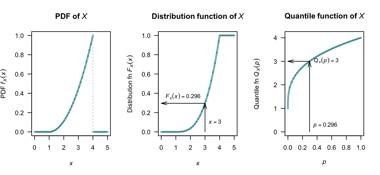
FIGURE 4.13: Left: the probability function of \(X\). Centre: the distribution function. Right: the quantile function for \(X\).
Example 4.26 (Quantile function: continuous rv) Consider the probability density function for a continuous random variable \(X\) such that \[ f_X(x) = 2\exp(-2x) \qquad \text{for $x > 0$} \] so that the distribution function is: \[ F_X(x) = \begin{cases} 0 & \text{for $x < 0$}\\ 1 - \exp(-2x) & \text{for $x \ge 0 $}. \end{cases} \] For \(0 < p < 1\), the quantile function \(Q_X(p)\) is found by solving \(F_X(x) = p\); i.e., the solution to \(p = 1 - \exp(-2x)\). This yields \[ Q_X(p) = F_X^{-1}(p) = -\frac{1}{2}\log(1 - p) \] for \(0 \le p \le 1\). For example, three quarters of the probability occurs before \[ Q_X(3/4) = -\frac{1}{2}\log\big(1 - (3/4)\big) = \frac{\log 4}{2} = 0.6931\dots \] In other words, \(75\)% of the probability occurs at or below \(x \approx 0.6931\); see Fig. 4.14.
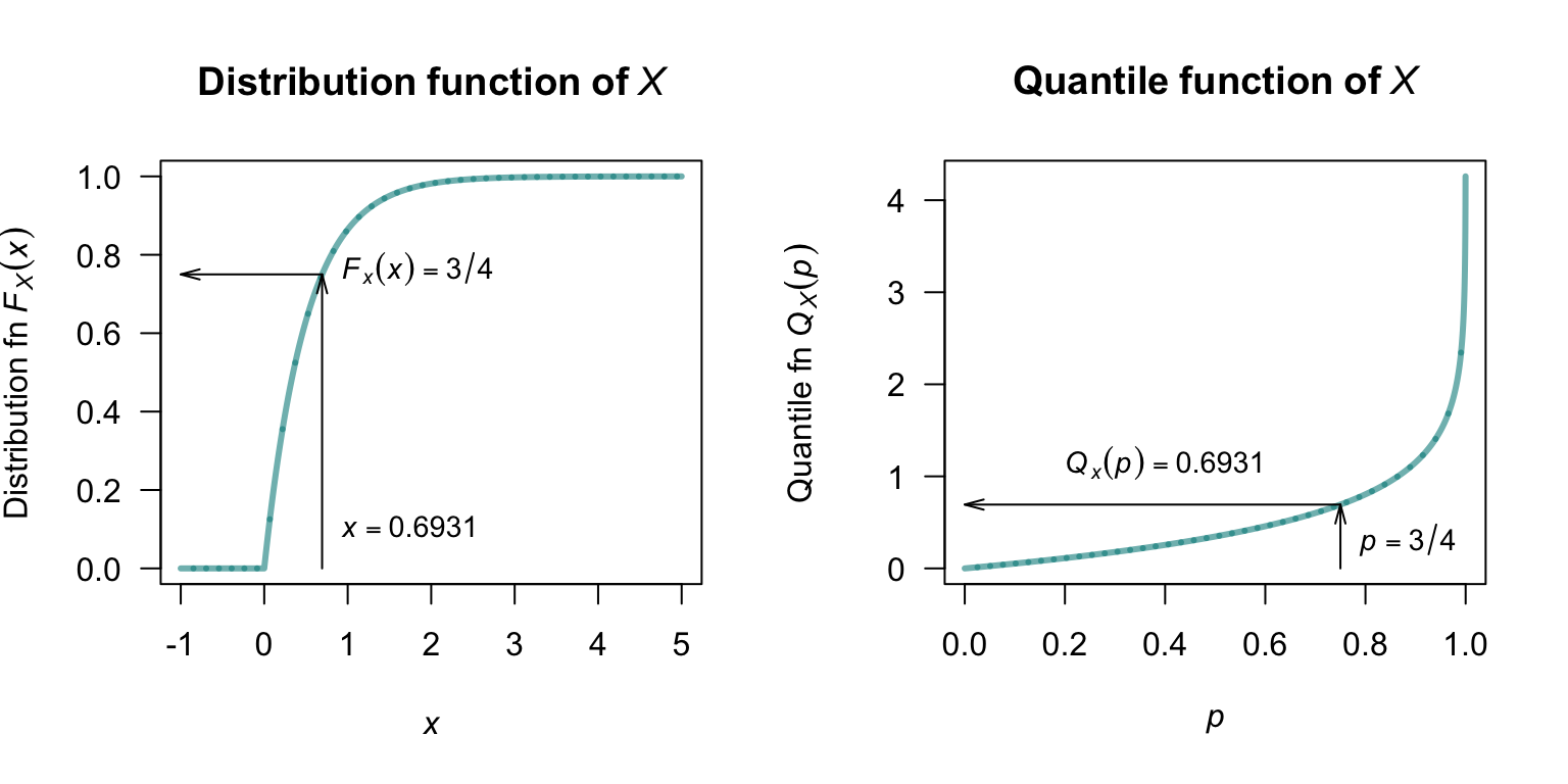
FIGURE 4.14: Left: the distribution function of \(X\). Right: the quantile function for \(X\).
When \(X\) is a discrete random variable, and so the distribution function is discontinuous, great care is needed when applying Eq. (4.4).
Example 4.27 (Quantile function: discrete rv) Consider the discrete random variable in Example 4.21, for which \[ F_X(x) = \begin{cases} 0 & \text{for $x < 10$;}\\ 0.1 & \text{for $10 \le x < 11$;}\\ 0.4 & \text{for $11 \le x < 15$;}\\ 0.8 & \text{for $15 \le x < 17$;}\\ 1 & \text{for $x \ge 17$,} \end{cases} \] as shown in Fig. 4.15 (left panel).
The quantile function is found by solving \(F_X(x) \ge p\) for \(0 < p \le 1\). This gives: \[ Q_X(p) = \begin{cases} 10 & \text{for $0 < p \le 0.1$;}\\ 11 & \text{for $0.1 < p \le 0.4$;}\\ 15 & \text{for $0.4 < p \le 0.8$;}\\ 17 & \text{for $0.8 < p \le 1$.} \end{cases} \] as shown in Fig. 4.15. For example, \(Q_X(0.02) = 10\) and \(Q_X(0.3) = 11\).
In addition, \(Q_X(0.4) = 11\), because \(11\) is the smallest value such that \(F_X(x) \ge 0.4\). Also, while \(F_X(15) = 0.9\), \(11\) is the infimum. Similarly, \(Q_X(1) = 17\).
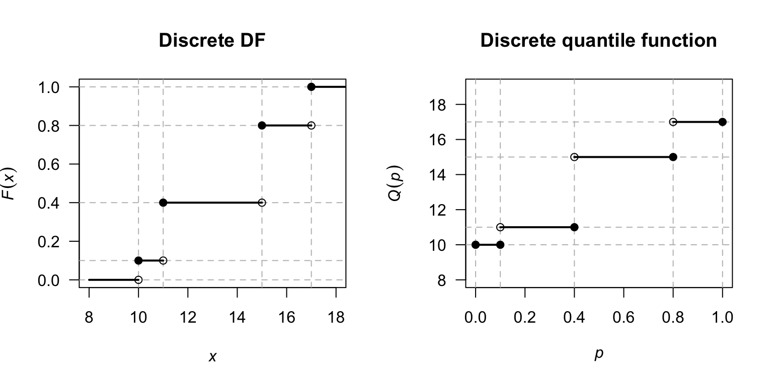
FIGURE 4.15: Left: the distribution function of \(X\). Right: the quantile function of \(X\).
For the discrete variable \(X\) above, \(Q_X(1) = 17\) because \(17\) is the smallest value such that \(F_X(x)\) reaches \(1\). For \(Q_X(0)\), we observe that while \(F_X(x) = 0\) for all \(x < 10\), the ‘first’ point to provide any probability is \(x = 10\), making it the most common choice for \(Q_X(0)\).
If the distribution has a clear end (like the random variable \(X\) in Example 4.27, where no furtehr probability is added after \(X = 17\)), \(Q(1)\) is just that end point. If the distribution has a tail that goes on forever (like the random variable \(X\) in Example 4.26), \(Q(1)\) is infinity.
| Continuous example | Discrete example | |
|---|---|---|
| Support | \([0, \infty)\) (unbounded) | \(\{10, 11, 15, 17\}\) (bounded) |
| \(Q(0)\) calculation | \(\inf\{ x\mid 1 - \exp(-2x)\ge 0\} = 0\) | \(\min\{10, 11, 15, 17\} = 10\) |
| \(Q(1)\) calculation | \(\inf\{ x\mid 1 - \exp(-2x) = 1\} = \infty\) | \(\inf\{x \mid F_X(x) = 1\} = 17\) |
| Limit \(p\to 1\) | \(Q(p)\to \infty\) | \(Q(p) = 17\) for all \(p > 0.9\) |
| Visually | Smooth curve that | A series of steps that |
| never quite reaches \(1\) | ends at a top landing |
A mixed random variable has a distribution function \(F_X(x)\) that contains both continuous slopes and discrete jumps. The quantile function \(Q_X(p)\) still follows the definition in Eq. (4.4).
Example 4.28 (Quantile function: mixed rv) Consider a random variable \(X\) that represents a censored waiting time. There is a \(50\)% chance the event happens instantly (so that \(x = 0\)), and a \(50\)% chance it follows the continuous distribution \[ f_X(x) = \exp(-x) \qquad\text{for $x \ge 0$}. \] The distribution function (Fig. 4.16, left panel) is: \[ F_X(x) = \begin{cases} 0 & \text{for $x < 0$} \\ 0.5 + 0.5\left(1 - \exp(-x)\right) & \text{for $x \ge 0$}. \end{cases} \] At \(x = 0\), the DF jumps from \(F_X(x) = 0\) to \(F_X(x) = 0.5\).
To find the quantile function, we look for the smallest value of \(x\) such that \(F_X(x) \ge p\):
- For \(0 < p \le 0.5\): The smallest \(x\) that satisfies \(F_X(x) \ge p\) is exactly \(x = 0\), because \(F_X(0) = 0.5\), which is \(\ge p\) for all these values.
- For \(0.5 < p < 1\): Solving \(0.5 + 0.5\left(1 - \exp(-x)\right) = p\) gives \(x = -\log\left(2(1 - p)\right)\).
The resulting quantile function (Fig. 4.16, right panel) is: \[ Q_X(p) = \begin{cases} 0 & \text{for $0 < p \le 0.5$} \\ -\log\left(2(1 -p)\right) & \text{for $0.5 < p < 1$}. \end{cases} \]
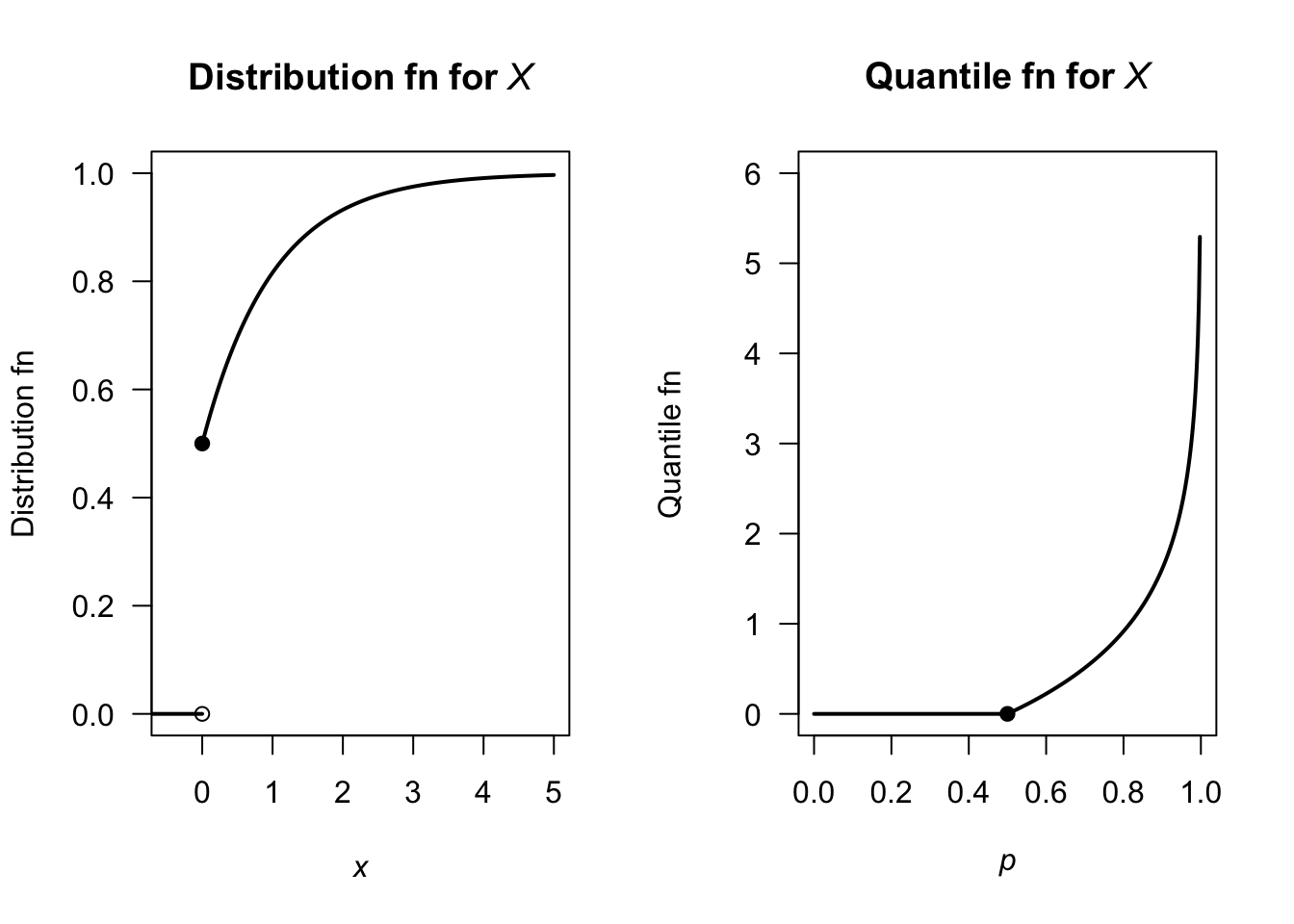
FIGURE 4.16: The distribution function (left) and quantile function (right) for the random variable \(X\).
4.7 Generating random numbers
Generating random numbers from a specified distribution is fundamental to simulations of real-world scenarios. However, computers often will only have the capacity to generatie (pseudo-)random numbers between \(0\) and \(1\), even though random numbers from other distributions are often more useful in computer modelling and simulation (for example, Sects. 6.10 and 7.9). For instance, generating heights of people at random may require the heights to have bell-shaped distribution, with an average value of (say) \(180\,\text{cm}\), with most heights between about \(175\,\text{cm}\) and \(185\,\text{cm}\), but a few smaller than \(175\,\text{cm}\) and a few larger than \(185\,\text{cm}\).
Computer software can generally provide random numbers between \(0\) and \(1\), which correspond to the range of \(F_X(x)\), or equivalently the domain of \(Q_X(p)\), for any random variable \(X\). Suppose a random number \(p^*\) is chosen between \(0\) and \(1\); then, the quantile function is used to find the corresponding value \(x^*\): \[ x^* = Q_X(p^*) \] (see Fig. 4.17). By repeating this process with many different random values of \(p^*\), we naturally generate more \(x\) values in regions where the distribution function is steep (high density) and fewer \(x\) values where the distribution function is flat (low density).
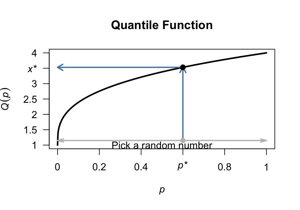
FIGURE 4.17: Selecting a random number from some distribution, using the quantile function.
In R, random numbers between \(0\) and \(1\) are found using the function runif():
runif(10) # '10' here means to generate 10 random numbers between 0 and 1
#>  [1] 0.2516103 0.5757754 0.0141046 0.8898474 0.5825408 0.4986948
#>  [7] 0.8753130 0.3948804 0.3206488 0.2908654
Example 4.29 (Random numbers from a continuous distribution) Random numbers from the distribution \[ f_X(x) = 2 \exp(-2x)\quad\text{for $x > 0$}, \] as in Example 4.26, can be generated using R using this idea:
# Create an R function for the quantile function
quantileFn <- function(p){ -log(1 - p) / 2}

# Create 20 random numbers between 0 and 1
rnos <- runif(20)

# Random numbers from the specified distribution
rSpecified <- quantileFn(rnos)
rSpecified
#>  [1] 2.171700641 0.473694652 0.029182963 0.331987237 0.300095204
#>  [6] 0.017917478 0.005156677 0.322064849 0.287240059 0.145286330
#> [11] 0.504798971 0.224026252 0.108944868 0.370482873 0.043328258
#> [16] 0.979405812 1.083842484 0.545094388 0.386174984 0.044326855
4.8 Statistical computing with probability functions
4.8.1 Discrete random variables
In Example 4.21, the random variable \(X\) was stated to have the PMF \[ f_X(x) = \begin{cases} 0.1 & \text{for $x = 10$};\\ 0.3 & \text{for $x = 11$};\\ 0.5 & \text{for $x = 15$};\\ 0.1 & \text{for $x = 17$}. \end{cases} \] In R, define the values of \(X\) where probabilities are non-zero:
Then the probability mass function is
data.frame(x, p)
#>    x   p
#> 1 10 0.1
#> 2 11 0.3
#> 3 15 0.5
#> 4 17 0.1
This is a valid PMF, as the probabilities sum to one:
sum(p)
#> [1] 1
The DF can be found using the function cumsum(), the cumulative summation:
F <- cumsum(p)
data.frame(x, F)
#>    x   F
#> 1 10 0.1
#> 2 11 0.4
#> 3 15 0.9
#> 4 17 1.0
This agrees with the DF given earlier in Example 4.21.
4.8.2 Continuous random variables
In Example 4.15, the continuous random variable \(W\) was given with the PDF
\[
f_W(w) =
2w \qquad \text{for $0 < w < 1$}.\\
\]
The PDF can be expressed in R as a function (note that the integrate() function in R, used below, always denotes the random variable by x):
fW <- function(x) {2 * x}Then, the PDF can be plotted (Fig. 4.18, left panel) using:
curve(fW,
      main = "Density function",  # Main title
      xlab = "w",      # Horizontal-axis label
      ylab = "PDF",    # Vertical-axis label
      from = 0,        # Lower x-value of plot
      to = 1,          # Upper x-value of plot
      las = 1,         # Horizontal axis labels
      lwd = 3)         # Lines a little thicker
As required, the total area under the curve is \(1\):
integrate(fW,
          lower = 0,         # Lower limit of integration
          upper = 1)$value   # Upper limit of integration
#> [1] 1
Probabilities can be found similarly; for example, to find \(\Pr(0.2 < X < 0.6)\):
integrate(fW,
          lower = 0.2,
          upper = 0.6)$value
#> [1] 0.32
The DF can also be defined (Vectorize() is an R construct to avoids writing loops):
FW <- Vectorize(function(x) {
        integrate(fW,                  # Integrate f(x)...
                  lower = 0,           # ... from 0 to x
                  upper = x)$value})   # Return the *value*
The DF can be plotted also (Fig. 4.18, right panel):
curve(FW,
      main = "Distribution function",  # Main title
      xlab = "w",       # Horizontal-axis label
      ylab = "DF",     # Vertical-axis label
      from = 0,         # Lower x-value of plot
      to = 1,           # Upper x-value of plot
      las = 1,          # Axis labels horizontal
      lwd = 3)          # Lines a little thicker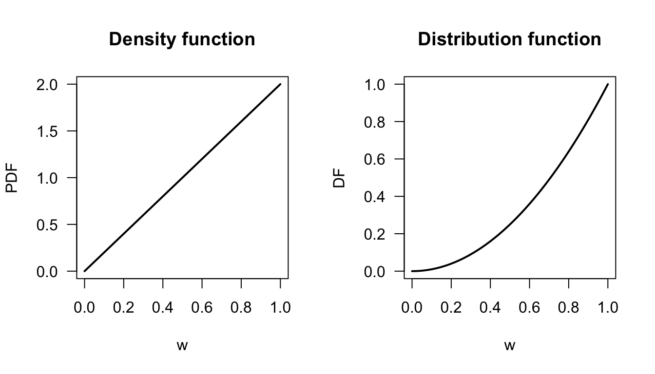
FIGURE 4.18: The density function and distribution function for \(W\), produced by R.
Then, \(\Pr(0.2 < W < 0.6)\) can be found using the distribution function:
FW(0.6) - FW(0.2)
#> [1] 0.32
4.8.3 Empirical probability functions
When random numbers are generated from a probability distribution, the resulting numbers are called a sample, and can be used as an estimate of the the probability function of the distribution. The estimated probability function is called an empirical probability function.
For a continuous distribution, a histogram of the simulated values estimates the probability density function.
The histogram divides the range of the data into bins and counts the number of values in each bin; when scaled so that the total area equals \(1\), the histogram approximates the PDF.
In R, hist(x, freq = FALSE) produces this scaled histogram.
The larger the number of simulated values, the closer the empirical probability function is to the true theoretical probability function.
For a discrete distribution, a bar chart of the relative frequencies of the simulated values estimates the PMF.
In R, table(x) / length(x) computes the relative frequencies, and barplot() displays them.
For a mixed distribution, the empirical probability function combines both: a solid dot at \(x = 0\) shows the simulated proportion of zeros (estimating the probability mass \(\Pr(X = 0)\)), and a histogram of the positive values estimates the continuous component of the density.
Example 4.30 (Empirical probability density) In Example 4.29, \(20\) random numbers were generated from the continuous probability density function \(f_X(x) = 2 \exp(-2x)\) for \(x > 0\). To generate and display \(n = 50\) random numbers in R:
rnos <- runif(20)
x <- quantileFn(x)      # Function as defined previously
hist(x,
     freq   = FALSE)    # Ensures a scaled histogram
The empirical probability density function for increasing values of \(n\) are show in Fig. 4.19. The empirical probability function is closer to the actual probability density function as \(n\) increases.
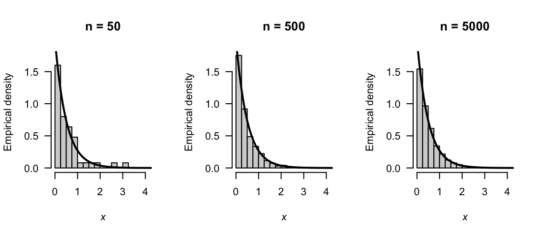
FIGURE 4.19: Empirical probability density functions based on samples of size \(n = 50\), \(500\), and \(5000\). As \(n\) increases, the empirical probability density function converges to the theoretical PDF (shown as solid lines).
Example 4.31 (Empirical probability density) Consider generating random numbers from the discrete probability mass function \[ p_X(x) = 0.6\cdot 0.4^x\quad\text{for $x = 0, 1, 2, \dots$} \] The distribution function is \[ F_X(x) = 1 - 0.4^{x + 1}, \] so the quantile function is found by solving \[ 1 - 0.4^{x + 1} \ge p, \] giving \[ Q_X(p) = \left\lceil \frac{\log(1 - p)}{\log 0.4} - 1 \right\rceil \quad\text{for $0 \le p \le 1$}, \] where \(\lceil x \rceil\) is the ceiling function: the smallest integer not less than \(x\) (e.g., \(\lceil\pi\rceil = 4\) and \(\lceil-\pi\rceil = -3\)).
To generate and display \(n = 50\) random numbers in R:
rnos <- runif(20)
quanFn <- function(p) {
  ceiling( log(1 - p)/log(0.4) - 1 )
  }
x <- quanFn(rnos)
barplot( table(x))
The empirical probability mass function for increasing values of \(n\) are show in Fig. 4.20. The empirical probability function is closer to the actual probability mass function as \(n\) increases.
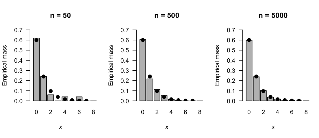
FIGURE 4.20: Empirical probability mass functions based on samples of size \(n = 50\), \(500\), and \(5000\). As \(n\) increases, the empirical probability mass function converges to the theoretical PMF (shown as the solid dots).
4.9 Exercises
Selected answers appear in Sect. F.3.
Exercise 4.1 For the following random processes, determine the range \(\mathcal{R}_X\) and define the random variable of interest. Determine whether the random variable is discrete, continuous or mixed. Justify your answer.
- The number of heads in two throws of a fair coin.
- The number of throws of a fair coin until a head is observed.
- The time taken to download a webpage.
- The time it takes to walk to work.
Exercise 4.2 For the following random processes, determine the range \(\mathcal{R}_X\) and define the random variable of interest. Determine whether the random variable is discrete, continuous or mixed. Justify your answer.
- The number of cars that pass through an intersection during a day.
- The number of X-rays taken at a hospital per day.
- The barometric pressure in a given city at \(5\)pm each afternoon.
- The length of a phone call connection.
Exercise 4.3 Consider the random variable \(Y\) with the probability density function shown in Fig. 4.21 (left panel). Find the value(s) of \(a\) so that this represents a valid probability function.
Exercise 4.4 Consider the random variable \(T\) with the probability density function shown in Fig. 4.21 (right panel). Find the value(s) of \(a\) so that this represents a valid probability function.
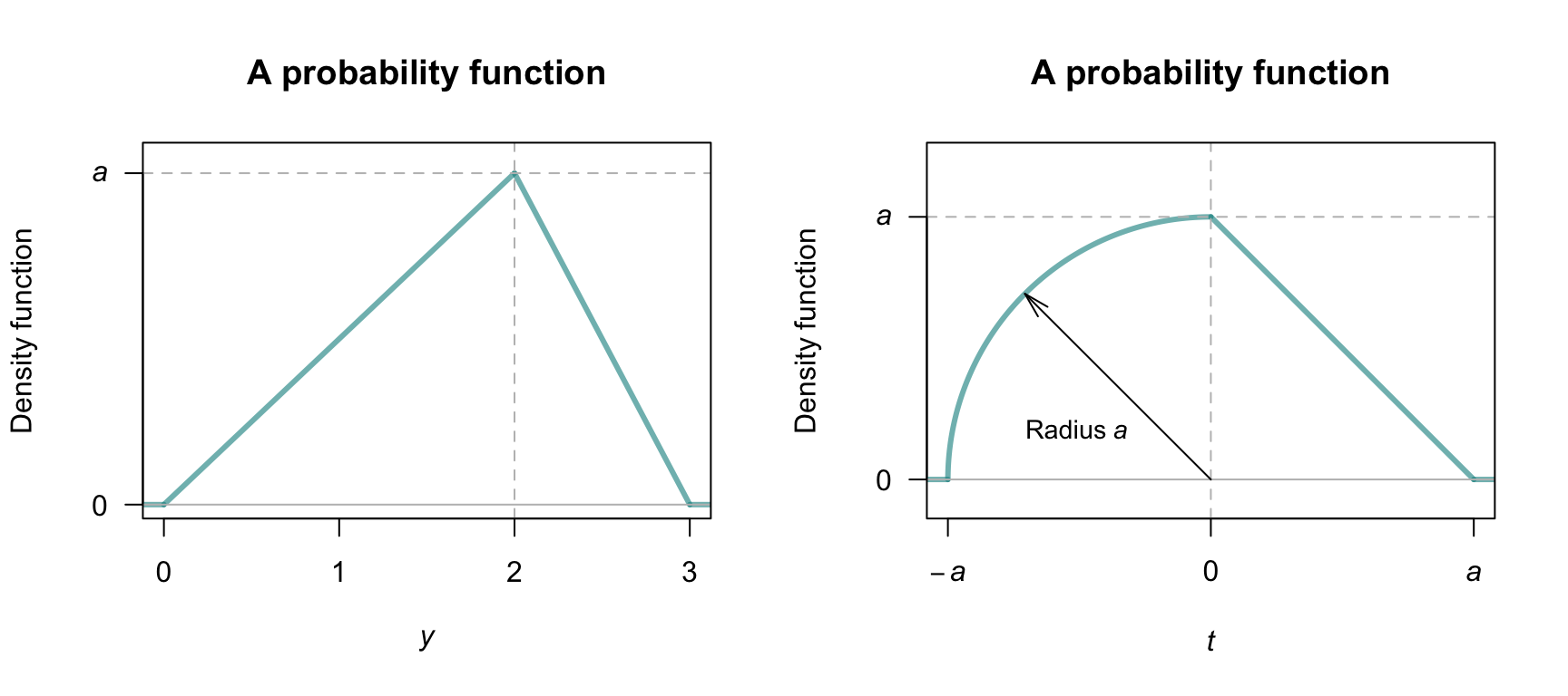
FIGURE 4.21: Two probability density functions
Exercise 4.5 The random variable \(X\) has the probability function \[ p_X(x) = \begin{cases} 0.3 & \text{for $x = 10$};\\ 0.2 & \text{for $x = 15$};\\ 0.5 & \text{for $x = 20$}. \end{cases} \]
- Show that \(p_X(x)\) is a valid probability distribution.
- Plot the probability function of \(X\).
- Find and plot the distribution function for \(X\).
- Find and plot the survival function for \(X\).
- Compute \(\Pr(X > 13)\).
- Compute \(\Pr(X \le 10 \mid X\le 15)\).
- Find and plot the quantile function. Show that your quantile function gives the correct values for \(Q_X(0)\) and \(Q_X(1)\).
Exercise 4.6 The random variable \(X\) has the probability mass function \[ p_X(x) = 2^{-x} \qquad \text{for $x = 1, 2, 3, \dots$}. \]
- Show that \(p_X(x)\) is a valid probability distribution.
- Plot the probability function of \(X\).
- Find and plot the distribution function for \(X\).
- Find and plot the survival function for \(X\).
- Compute \(\Pr(X < 4)\).
- Compute \(\Pr(X \le 2 \mid X\le 5)\).
- Find and plot the quantile function. Show that your quantile function gives the correct values for \(Q_X(0)\) and \(Q_X(1)\).
Exercise 4.7 Consider the continuous random variable \(X\) with probability function \[ f_Z(z) = (2z + 1)/4 \qquad \text{for $1 < z < 2$}. \]
- Plot the probability function of \(Z\).
- Find and plot the distribution function of \(Z\).
- Find and plot the survival function of \(Z\).
- Find \(\Pr(Z < 0)\).
- Find and plot the quantile function. Show that your quantile function gives the correct values for \(Q_Z(0)\) and \(Q_Z(1)\).
- Determine \(Q_Z(0.25)\).
Exercise 4.8 Consider the continuous random variable \(Z\) with probability function \[ f_Z(z) = \alpha (3 - z) \qquad \text{for $-1 < z < 2$}. \]
- Find the value of \(\alpha\).
- Plot the probability function of \(Z\).
- Find and plot the distribution function of \(Z\).
- Find and plot the survival function of \(Z\).
- Find \(\Pr(Z < 0)\).
- Find and plot the quantile function. Show that your quantile function gives the correct values for \(Q_Z(0)\) and \(Q_Z(1)\).
- Determine \(Q_Z(0.25)\).
Exercise 4.9 Consider the continuous random variable \(Y\) with probability density function \[ f_Y(y) = \frac{1}{2\sqrt{y + 1}} \quad \text{for $0 < y < 3$}. \]
- Plot the probability function of \(Y\).
- Find and plot the distribution function of \(Y\).
- Find and plot the survival function of \(Y\).
- Find \(\Pr( |Y - 1| < 1)\).
- Find and plot the quantile function. Show that your quantile function gives the correct values for \(Q_Y(0)\) and \(Q_Y(1)\).
- Determine \(Q_Y(0.5)\).
Exercise 4.10 Consider the continuous random variable \(X\) with probability density function \[ f_X(x) = \frac{16 + x^2}{51} \quad \text{for $-2 < x < 1$}. \]
- Plot the probability function of \(X\).
- Find and plot the distribution function of \(X\).
- Find and plot the survival function of \(X\).
- Find \(\Pr(X < 3)\).
- Find and plot the quantile function. Show that your quantile function gives the correct values for \(Q_X(0)\) and \(Q_X(1)\).
- Determine \(Q_X(0.5)\).
Exercise 4.11 The random variable \(T\) is defined as shown in Fig. 4.22 (left panel).
- Determine the formula for the PDF for \(T\).
- Determine and plot the DF for \(T\).
- Determine and plot the survival function for \(T\).
- Determine and plot the quantile function for \(T\).
Exercise 4.12 The random variable \(Z\) is defined as shown in Fig. 4.22 (right panel).
- Determine the formula for the PDF for \(Z\).
- Determine and plot the DF for \(Z\).
- Determine and plot the survival function for \(Z\).
- Determine and plot the quantile function for \(Z\).
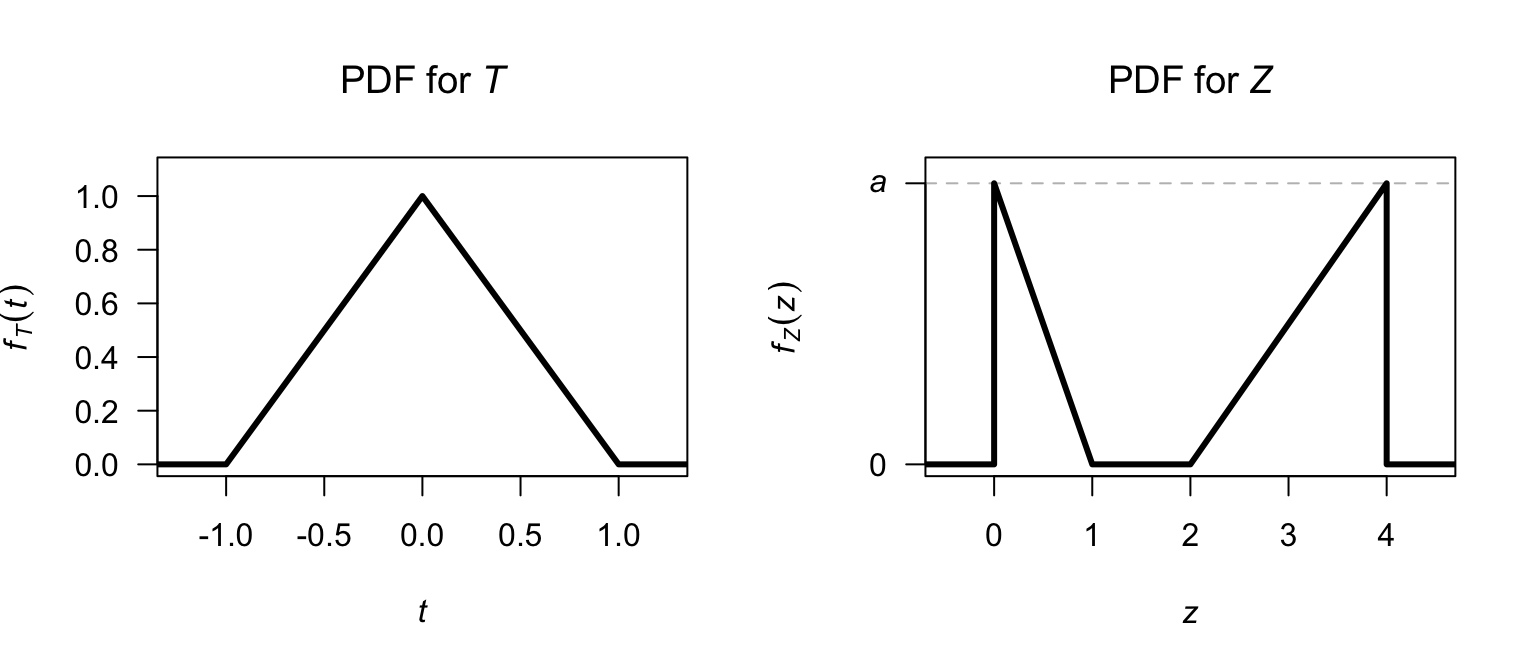
FIGURE 4.22: The PDF for \(T\) (left) and \(Z\) (right).
Exercise 4.13 Let \(Y\) be a continuous random variable with PDF \[ f_Y(y) = a(1 - y)^2,\quad \text{for $0\le y\le 1$}. \]
- Show that \(a = 3\).
- Find \(\Pr\left(| Y - \frac{1}{2}| > \frac{1}{4} \right)\).
- Use R to draw a graph of \(f_Y(y)\) and show the area described above.
Exercise 4.14 Suppose the random variable \(Y\) has the PDF \[ f_Y(y) = \begin{cases} \frac{2}{3}(y - 1) & \text{for $1 < y < 2$};\\[3pt] \frac{2}{3} & \text{for $2 \le y < 3$}. \end{cases} \]
- Plot the PDF.
- Determine the DF.
- Confirms that the DF is a valid DF.
Exercise 4.15 Consider the continuous radom variable \(X\) with pdf \[ f_X(x) = \sin(x)\quad\text{for $0 < x < (\pi/2)$.} \]
- Determine and plot the DF for \(X\).
- Determine and plot the survival function for \(X\).
- Determine and plot the quantile function for \(X\).
Exercise 4.16 Consider the continuous radom variable \(Y\) with pdf \[ f_Y(y) = \exp(-|y|)/2\quad\text{for $-\infty < y < \infty$.} \]
- Determine and plot the DF for \(Y\).
- Determine and plot the survival function for \(Y\).
- Determine and plot the quantile function for \(Y\).
Exercise 4.17 Consider the mixed random variable \(Y\) with probability function \[ f_Y(y) = \begin{cases} p & \text{for $y = 0$};\\ 1 - y & \text{for $0 < y < 1$}. \end{cases} \]
- Find the value of \(p\).
- Carefully plot the probability function of \(Y\).
- Find and carefully plot the distribution function of \(Y\).
- Find and carefully plot the survival function of \(Y\).
- Find \(\Pr(Y < 0.5)\).
- Find and carefully plot the quantile function of \(Y\).
Exercise 4.18 Consider the mixed random variable \(X\) with probability function \[ f_X(x) = \begin{cases} c & \text{for $x = 0$};\\ x/2 & \text{for $0 < x < 1$};\\ (3 - x)/4 & \text{for $1 < x < 3$}. \end{cases} \]
- Find the value of \(c\).
- Carefully plot the probability function of \(X\).
- Find and plot the distribution function of \(X\).
- Find and carefully plot the survival function of \(X\).
- Find \(\Pr(X > 1)\).
- Find and carefully plot the quantile function of \(X\).
Exercise 4.19 Consider the mixed random variable \(X\) with probability function \[ f_X(x) = \begin{cases} a & \text{for $x = 0$};\\ a - x & \text{for $0 < x < a$}. \end{cases} \]
- Find the value of \(a\).
- Carefully plot the probability function of \(X\).
- Find and carefully plot the distribution function of \(X\).
- Find and carefully plot the survival function of \(X\).
- Find and carefully plot the quantile function of \(X\).
Exercise 4.20 Consider the mixed random variable \(Y\) with probability function \[ f_Y(y) = \begin{cases} c & \text{for $y = 0$};\\ c(2 - y^2) & \text{for $0 < y < 1$}. \end{cases} \]
- Find the value of \(c\).
- Carefully plot the probability function of \(Y\).
- Find and carefully plot the distribution function of \(Y\).
- Find and carefully plot the survival function of \(Y\).
- Find and carefully plot the quantile function of \(Y\).
Exercise 4.21 Consider the random variable \(Y\) with the probability mass function \[ f_Y(y) = y^\alpha \qquad \text{for $y = 2, 4$}. \] Find the value(s) of \(\alpha\) so that \(f_Y(y)\) is a valid probability function.
Exercise 4.22 Consider the random variable \(X\) with the probability mass function \[ f_X(x) = x + 1 \qquad \text{for $x = b, b + 1, b + 2$}. \] Find the value(s) of \(b\) so that \(f_X(x)\) is a valid probability function.
Exercise 4.23 Consider the discrete random variable \(W\) with DF \[ F_W(w) = \begin{cases} 0 & \text{for $w < 10$};\\ 0.3 & \text{for $10 \le w < 20$};\\ 0.7 & \text{for $20 \le w < 30$};\\ 0.9 & \text{for $30 \le w < 40$};\\ 1 & \text{for $w \ge 40$}. \end{cases} \]
- Find and plot the PMF of \(W\).
- Compute \(\Pr(W < 25)\) using the PMF, and using the DF.
Exercise 4.24 Consider the continuous random variable \(Y\) with DF \[ F_Y(y) = \begin{cases} 0 & \text{for $y \le 0$};\\ y(4 - y^2)/3 & \text{for $0 < y < 1$};\\ 1 & \text{for $y \ge 1$}. \end{cases} \]
- Find and plot the PDF of \(Y\).
- Compute \(\Pr(Y < 0.5)\) using the PDF and using the DF.
Exercise 4.25 A study of the service life of concrete in various conditions (Liu and Shi 2012) used the following distribution for the chlorine threshold of concrete1: \[ f(x; a, b, c) = \begin{cases} \displaystyle \frac{2(x - a)}{(b - a)(c - a)} & \text{for $a\le x\le c$}\\[6pt] \displaystyle \frac{2(b - x)}{(b - a)(b - c)} & \text{for $c\le x\le b$} \end{cases} \] where \(c\) is the mode, and \(a\) and \(b\) are the lower and upper limits.
- Show that the distribution is a valid PDF. (This is easier geometrically than using integration.)
- Previous studies, cited in the article, suggest the values \(a = 0.6\) and \(c = 5\), and that the distribution is symmetric. Write down the PDF for this case.
- Determine the DF using the values above.
- Plot the PDF and DF.
- Determine \(\Pr(X > 3)\).
- Determine \(\Pr(X > 3 \mid X > 1)\).
- Explain the difference in meaning for the last two answers.
Exercise 4.26 In a study modelling waiting times at a hospital (Khadem et al. 2008), patients are classified into one of three categories: Red (critically ill or injured patients), Yellow (moderately ill or injured patients), or Green (injured or uninjured patients).
For Yellow patients, the service time of doctors are modelled using a triangular distribution, with a minimum at \(3.5\,\text{mins}\), a maximum at \(30.5\,\text{mins}\) and a mode at \(5\,\text{mins}\).
- Plot the PDF and DF.
- If \(S\) is the service time, compute \(\Pr(S > 20 \mid S > 10)\).
Exercise 4.27 In meteorology and climatology, rainfall is often graphed using rainfall survival functions (Dunn 2001) \(S_X(x) = 1 - F_X(x)\), where \(X\) represents the rainfall.
- Explain what is measured by \(S_X(x)\) in this context, and explain why it may be more useful than just \(F_X(x)\) when studying rainfall.
- The data in Table 4.4 shows the total monthly rainfall at Charleville, Queensland, from 1942 until 2022 for the months of June and December. (Data supplied by the Bureau of Meteorology.) Plot \(S_X(x)\) for this rainfall data for each month on the same graph.
- Suppose a producer requires at least \(50\,\text{mm}\) of rain in June to plant a crop. Find the probability of this occurring from the plot above.
- Determine the median monthly rainfall in Charleville in June and December.
- Decide if the mean or the median is an appropriate measure of central tendency, giving reasons for your answer.
- Compare the probabilities of obtaining \(30\,\text{mm}\), \(50\,\text{mm}\), \(100\,\text{mm}\) and \(150\,\text{mm}\) of rain in the months of June and December.
- Write a one-or two-paragraph explanation of how to use diagrams like that presented here. The explanation should be aimed at producers (that is, experts in farming, but not in statistics) and should be able to demonstrate the usefulness of such graphs in decision making. Your explanation should be clear and without jargon. Use diagrams if necessary.
| June | December | |
|---|---|---|
| Zero rainfall | 3 | 0 |
| Over 0 to under 20 | 41 | 17 |
| 20 to under 40 | 19 | 17 |
| 40 to under 60 | 12 | 21 |
| 60 to under 80 | 2 | 9 |
| 80 to under 100 | 2 | 6 |
| 100 to under 120 | 0 | 3 |
| 120 to under 140 | 2 | 1 |
| 140 to under 160 | 0 | 4 |
| 160 to under 180 | 0 | 0 |
| 180 to under 200 | 0 | 1 |
| 200 to under 220 | 0 | 1 |
Exercise 4.28 Five people, including you and a friend, line up at random. The random variable \(X\) denotes the number of people between yourself and your friend. Determine the probability function of \(X\).
Exercise 4.29 Suppose a dealer deals four cards from a standard \(52\)-card pack. Define \(Y\) as the number of suits in the four cards. Deduce the distribution of \(Y\).
Exercise 4.30 To detect disease in a population through a blood test, usually every individual is tested. If the disease is uncommon, however, an alternative method is often more efficient.
In the alternative method (called a pooled test), blood from \(n\) individuals is combined, and one test is conducted. If the test returns a negative result, then none of the \(n\) people have the disease; if the test returns a positive result, all \(n\) individuals are then tested individually to identify which individual(s) have the disease.
Suppose a disease occurs in an unknown proportion of people \(p\) of people. Let \(X\) be the number of tests to be performed for a group of \(n\) individuals using the pooled test approach.
- Determine the sample space for \(X\).
- Deduce the probability distribution of the random variable \(X\).
Exercise 4.31 In a deck of cards, consider an Ace as high, and all picture cards (i.e., Jacks, Queens, Kings, Aces) as worth ten points. All other cards are worth their face value (i.e., an 8 is worth eight points.)
Deduce the probability distribution of the absolute difference between the value of two cards drawn at random from a well-shuffled deck of \(52\) cards.
Exercise 4.32 The leading digits of natural data that span many orders of magnitude (e.g., lengths of rivers; populations of countries) often follow Benford’s law. Numbers are said to satisfy Benford’s law if the leading digit, say \(d\) (for \(d\in \{1, \dots, 9\}\)) has the probability mass function \[ p_D(d) = \log_{10}\left( \frac{d + 1}{d} \right). \]
- Plot the probability mass function of \(D\).
- Compute and plot the distribution function of \(D\).
Exercise 4.33 Consider the random variable \(X\) with PDF \[ f_X(x) = \displaystyle \frac{k}{\sqrt{x(1 - x)}} \qquad \text{for $0 < x < 1$} \] for some constant \(k\).
- Plot the density function.
- Determine, and then plot, the distribution function.
- Compute \(\Pr(X > 0.25)\).
Exercise 4.34 Consider the distribution function \[ F_X(x) = \begin{cases} 0 & \text{for $x < 0$};\\ \exp(-1/x) & \text{$x \ge 0$}. \end{cases} \]
- Show that this is a valid DF.
- Compute the PDF.
- Plot the DF and PDF.
Exercise 4.35 Consider the random variable \(T\) with the probability function \[ f_T(t) = \begin{cases} a & \text{for $t = 0$}; \\ \frac{2}{3} - (t - 1)^2 & \text{for $0 < t < 2$}. \end{cases} \]
- Determine the value of \(a\).
- Plot the probability function.
- Determine the distribution function.
- Plot the distribution function.
Exercise 4.36 Consider rolling a fair, six-sided die.
- Find the probability mass function for the number of rolls required to roll a total of at least four.
- Find the probability mass function for the number of rolls required to roll a total of exactly four.
Exercise 4.37 Consider the PDF \(f_X(x) = (a + bx)^2\) defined over \(-1 < x < 1\).
- Find the relationship between \(a\) and \(b\) that is required for \(f_X(x)\) to be. a valid PDF.
- Find the PDF if \(f_X(x) = 4\).
- Find the distribution function of \(X\).
- Determine the quantile function. Confirm this is correct for \(Q_X(0)\) and \(Q_X(1)\).
- Plot the PDF, DF and quantile function for \(X\).
Exercise 4.38 Using the discrete random variable \(X\) from Example 4.21:
- Calculate \(Q(0.05)\) manually.
- Calculate \(Q(0.4)\) manually.
- Calculate \(Q(0.41)\) manually.
- Then, use the
quantile()function in R to verify. - Why does \(Q(0.4)\) and \(Q(0.41)\) give different results?
Exercise 4.39 Consider the mixed variable \(Y\) where \(\Pr(Y = 0) = 0.2\).
- If you were to generate \(1\,000\) random observations from this distribution using the
QY_mixed(runif(1000))method, approximately how many of those observations would be exactly \(0\)? - Run the simulation in R and use
sum(sim_data == 0)to see how close you get to your prediction.
Exercise 4.40 Consider the PDF \(f_X(x) = 2x\) for \(0 < x < 1\).
- Predict whether \(Q(0.5)\) will be greater than, less than, or equal to \(0.5\).
- Look at the PDF plot. Is there more ‘area’ (probability) on the left side or the right side of the midpoint \(x = 0.5\)?
- Use your
uniroot()function or the mathematical inverse \(Q(p) = \sqrt{p}\) to find the exact value.