3 Probability

Upon completion of this chapter you should be able to:

• understand the concepts of probability, and apply rules of probability.
• define probability from using different methods and apply them to compute probabilities in various situations.
• apply the concepts of conditional probability and independence.
• differentiate between mutually exclusive events and independent events.
• apply Bayes’ Theorem.
• use combinations and permutations to compute the probabilities of various events involving counting problems.

3.1 Introduction

Probability is a way of describing how likely it is for things to occur: will it rain tomorrow? will my team win on the weekend? A foundation in set theory allows the idea of probability to be developed, since probability relies heavily on many of the ideas from set theory.

Building upon this foundation, probability relates to the outcomes of random processes (or random experiments).

Definition 3.1 (Random process) A random process (or random experiment) is a procedure that:

• can be repeated, in theory, indefinitely under essentially identical conditions; and
• has well-defined outcomes; and
• the outcome of any individual repetition is unpredictable.

Examples of simple random processes include tossing a coin, or rolling a die. While the outcome of any instance of a random process is unknown, the possible outcomes are known.

3.2 Sample spaces

When talking about probability, the universal set is the set of all possible outcomes that can result from a random process, and is usually denoted \(S\), \(\Omega\) or \(U\). In probability, a sample space is a special case of a universal set. The universal set is ‘all things we care about’, whereas the sample space is ‘all outcomes that can occur’.

Definition 3.2 (Sample space) A sample space (or event space, or outcome space) for a random process is a set of all possible outcomes from a random process, usually denoted by \(U\) (for the ‘universal set’), \(S\) or \(\Omega\).

Example 3.1 (Sample space) Consider rolling a die. The sample space is the set of all possible outcomes: \[ S = \{ 1, 2, 3, 4, 5, 6\}. \]

As with sets, the sample space may be finite, or countably infinite, or uncountably infinite. When the sample space is finite or countably infinite, the sample space is called discrete. If a sample space is an uncountably infinite set, the sample space is called continuous.

Example 3.2 (Discrete sample space) The sample space in Example 3.1 is discrete.

Example 3.3 (Continuous sample space) Consider the height of students. The sample space is continuous (see Example 2.14).

Sample spaces can also be a mixture of discrete and continuous sample spaces. In these sample spaces, part of the sample space is discrete, and part is continuous. The most common example is when the discrete component refers to \(0\) and the continuous part refers to the positive real numbers \(\mathbb{R}\).

Example 3.4 (Mixed sample space) Consider the random process where we observe the rainfall recorded on any given day, \(R\).

If no rain falls, the rainfall recorded is exactly \(R = 0\); this is the discrete component. However, if rain does fall, the exact amount cannot be recorded exactly; this is the continuous component.

The sample space is \[ S = \{0\}\cup \mathbb{R}. \] The sample space is mixed.

3.3 Events

3.3.1 Simple events

While the sample space defines the set of all possible outcomes, usually we are interested in just some of those elements of the sample space. Events are subsets of the sample space (and hence are also sets).

Definition 3.3 (Event) An event \(E\) is a subset of \(S\), and we write \(E \subseteq S\).

By this definition, \(S\) itself is an event. If the sample space is a finite or countable infinite set, then an event is a collection of sample points.

Example 3.5 (Events) Consider the simple random process of tossing a coin twice. The sample space is the set \[S = \{ HH, \quad HT, \quad TH, \quad TT\},\] where H represents tossing a head and T represents tossing a tail, and the pair lists the result of the two tosses in order.

We can define the event \(A\) as ‘tossing a head on the second toss’, and list the elements: \[A = \{ HH, \quad TH\};\] notice that \(A \subset S\) (i.e., \(A\) is a proper subset of \(S\)).

The event \(T\), defined as ‘the set of outcomes corresponding to tossing three heads’, is the null or empty set; no sample points have three heads. That is, \(T = \varnothing\).

Definition 3.4 (Simple (elementary) event) In a sample space with a finite or countable infinite number of elements, an simple event (or a elementary event) is an event with one sample point, that cannot be decomposed into smaller events.

Example 3.6 (Simple events) Consider observing the outcome on a single roll of a die (Example 3.1), where the sample space is the set of all possible outcomes: \[ S = \{ 1, 2, 3, 4, 5, 6\}. \] The six simple events are: \[ \begin{array}{lll} E_1 = \{1\}\ \text{(i.e., roll a 1)}; & E_2 = \{2\}\ \text{(i.e., roll a 2)}; & E_3 = \{3\}\ \text{(i.e., roll a 3)}; \\ E_2 = \{4\}\ \text{(i.e., roll a 4)}; & E_5 = \{5\}\ \text{(i.e., roll a 5)}; & E_6 = \{6\}\ \text{(i.e., roll a 6)}. \end{array} \]

An important concept is that of an occurrence of an event.

Definition 3.5 (Occurrence) An event \(A\) occurs on a particular trial of a random process if the outcome of the trial is an element of the subset \(A\) from the random process.

3.3.2 Compound events

Simple events are usually not of great interest; events of interest usually contain many elements of the sample space. These are called compound events.

Definition 3.6 (Compound event) A collection of simple events is called a compound event.

Since compound events, like all events, are sets, operations on existing sets (Sect.  2.5) can be used to define compound events.

Example 3.7 (Simple and compound events) Consider observing the outcome on a single roll of a die, as shown in Example 3.6. Define the event \(T\) as ‘numbers divisible by \(3\)’ and event \(D\) as ‘numbers divisible by \(2\)’. \(T\) and \(D\) are compound events: \[ T =\{E_3, E_6\} = \{3, 6 \} \quad \text{and} \quad D = \{E_2, E_4, E_6\} = \{2, 4, 6 \}. \]

The set operations in Sect. 2.5 apply to events, because events are sets. However, a different language is usually used, to indicate that events are real outcomes, whereas sets are for describing structures more widely and abstractly (Table 3.1). For example, ‘disjoint’ is used for sets (Sect. 2.5), whereas ‘mutually exclusive’ is used when referring to events.

Definition 3.7 (Mutually exclusive) Events \(A\) and \(B\) are mutually exclusive if, and only if, \(A\cap B = \varnothing\); that is, they have no outcomes in common. That is, Events \(A\) and \(B\) are mutually exclusive if the corresponding sets are disjoint.

TABLE 3.1: The language used in set theory and probability. The examples are based on the examples of rolling a six-sided die, where the possible outcomes are \(\{1, 2, 3, 4, 5, 6\}\), \(A = \{1, 2, 3\}\) and \(B = \{1, 6\}\).

Set theory	Probability	Example
Set	Event
Element of set \(x \in A\)	Simple events	\(\{1\}\)
Universal set, \(U\)	Sample space, \(S\)	\(\{1, 2, 3, 4, 5, 6\}\)
Subset \(A\subseteq S\)	\(A\) is an event in \(S\)
Union \(A\cup B\)	\(A\) or \(B\)	\(\{1, 2, 3, 6\}\)
Intersection \(A\cap B\)	\(A\) and \(B\)	\(\{1\}\)
Complement \(A^c\)	Not \(A\)	\(\{4, 5, 6\}\)
Empty set \(\varnothing\)	Impossible event
Disjoint sets	Mutually exclusive events
Set difference \(A\setminus B\)	\(A\) occurs, but not \(B\)

Example 3.8 (Tossing a coin twice) Consider the simple random process of tossing a coin twice (Example 3.5), and define events \(M\) and \(N\) as follows:

Event	Notation	Set of simple events
‘Obtain a Head on Toss 1’	\(M\)	\(\{HT, HH\}\)
‘Obtain a Tail on Toss 1’	\(N\)	\(\{TT, TH\}\)

The two sets are disjoint, as no sample points are common to \(M\) and \(N\). The two events are therefore mutually exclusive.

Since events are really just sets, the set algebra (Sect. 2.7) and the use of Venn diagrams (Sect. 2.6) applies to events also.

Example 3.9 (Rolling a die) Suppose we roll a single, six-sided die. For rolling a die, the sample space is \(S = \{1, 2, 3, 4, 5, 6\}\). We can define these two events: \[ \begin{array}{rcl} E = {} & \text{An even number is thrown} &= \{2, 4, \phantom{5, }6\};\\ G = {} & \text{A number larger than 3 is thrown} &= \{\phantom{2, }4, 5, 6\}. \end{array} \] Then, the following compound events could be defined: \[\begin{align*} E \cap G &= \{4, 6\} & E \cup G &= \{ 2, 4, 5, 6\}\\ E^c &= \{ 1, 3, 5\} & G^c &= \{ 1, 2, 3\}. \end{align*}\] We can make other observations too: \[\begin{align*} E \cap G^c &= \{2, 4, 6\} \cap \{ 1, 2, 3\} = \{ 2 \};\\ E^c \cap G^c &= \{1, 3, 5\} \cap \{ 1, 2, 3\} = \{ 1, 3 \}. \end{align*}\] See the Venn diagram in Fig. 3.1.

FIGURE 3.1: A Venn diagram showing events \(E\) and \(G\).

Example 3.10 (Throwing a cricket ball) Consider throwing a cricket ball, where the distance of the throw (in metres) is of interest. We could define the sample space \(D\) as \(D = \{ d \in \mathbb{R} \mid d \ge 0 \}\). More practically, we could write \[ D = \{ d \in \mathbb{R} \mid 0 < d < 150 \} \] given that throwing a cricket ball greater than \(150\,\text{m}\) is effectively impossible (and has never been recorded), and throwing a cricket ball exactly \(0\,\text{m}\) is also impossible in practice.

Two events can be defined: \[\begin{align*} B_1 &= \{b \in D \mid b \ge 40\} = [40, 150)\text{(i.e., throw a cricket ball at least $40\,\text{m}$)};\\ B_2 &= \{b \in D \mid b < 50\} = (0, 50) \text{(i.e., throw a cricket ball less than $50\,\text{m}$)}. \end{align*}\] (All events must be subsets of the sample space \(D\).) Then: \[\begin{align*} B_1 \cap B_2 &= \{b\in D \mid 40\le b < 50\}\quad \text{(i.e., throw the ball at least $40\,\text{m}$ but less than $50\,\text{m}$)};\\ B_1 \cup B_2 &= (0, 150) = D;\\ B_1^c &= \{b\in D \mid b < 40\}\quad \text{(i.e., throw the ball less than $40\,\text{m}$)}. \end{align*}\]

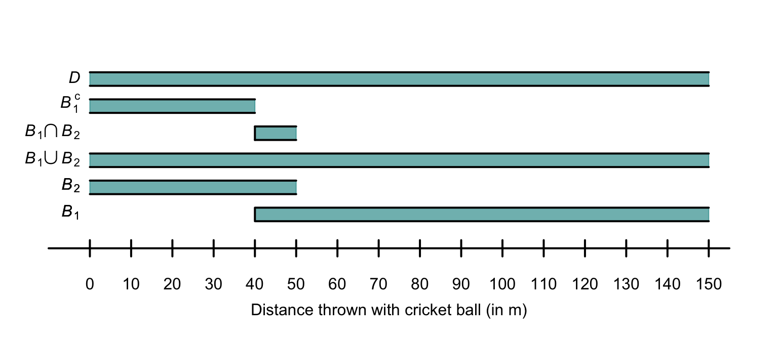
FIGURE 3.2: The two events \(B_1\) and \(B_2\) defined for throwing a cricket ball, the sample space \(D\), and three events defined with \(B_1\) and \(B_2\). When the bar representing the event is open at an end, the indicated value is included in the region.

3.4 Probablility

3.4.1 Definitions

Usually, we are interested in how likely it is for various outcomes from a random experiment to occur. That is, how likely it is to observe any of the various events defined on the sample space. Probability is the mathematical term for quantifying this likelihood. The probability of an event \(E\) occurring is denoted \(\text{Pr}(E)\).

Definition 3.8 (Probability) Probability is a function that assigns a number to an event. That is, for some event \(E\), the value \(\Pr(E)\) represents the probability that event \(E\) occurs.

The probability of an event \(E\) occurring can be denoted as \(\text{P}(E)\), \(\text{Pr}(E)\), \(\text{Pr}\{E\}\), \(\Pr[E]\), or using other similar notation.

This definition in Def. 3.8 allows any number to be assigned to an event, without rules or restrictions (‘assigns a number’). Some restrictions must be placed on the numbers that can be assigned to make this definition workable, practical and universally understood.

3.4.2 Three axioms of probability

While we have defined probability as a function that assigns a number to an event, we have not stated what numbers can be assigned as a ‘probability’. What values should a probability take? How should these numerical likelihoods be assigned?

A rigorous foundation for probability is found by using three fundamental axioms, called the Axioms of Probability. Using these axioms, all other rules about probability can be derived. These axioms formally define the rules that apply to all probabilities.

An axiom is a self-evident truth that does not require proof, or cannot be proven. They form the starting point for building further proofs.

Definition 3.9 (Kolmogorov's three axioms of probability) Consider a sample space \(S\) for a random process, and an event \(A\) in \(S\) so that \(A\subseteq S\). For every event \(A\) (a subset of \(S\)), a number \(\Pr(A)\) can be assigned which is called the probability of event \(A\).

Kolmogorov’s three axioms of probability are:

1. Non-negativity: \(\Pr(A) \ge 0\).
   The probability of any event is a non-negative real number.
2. Exhaustive: \(\Pr(S) = 1\).
   The event that something happens has probability \(1\), since the sample space lists all possible outcomes.
3. Additivity: If \(A_1\) and \(A_2\) are two mutually exclusive events in \(S\) (i.e., \(A_1 \cap A_2 = \varnothing\)), then \[ \Pr(A_1 \cup A_2) = \Pr(A_1) + \Pr(A_2). \]

3.4.3 Rules of probability

These purpose of these axioms is to formally define probability and the rules that apply to probabilities. These axioms of probability, and only these axioms, can be used to develop all other probability formulae. For example, these properties follow from these three axioms, for any Events \(A\) and \(B\) defined on a sample space \(S\):

• Bounds: \(0 \le \Pr(A)\le 1\); that is, probabilities are numbers between zero and one inclusive for any event \(A\).
• Empty sets: \(\Pr(\varnothing) = 0\); that is, the probability of an impossible event (with zero elements) is zero.
• Monotonicity: If \(A\subseteq B\), then \(\Pr(A) \le \Pr(B)\); that is, if every outcome in event \(A\) is also in event \(B\), then the probability of \(A\) cannot exceed the probability of \(B\).
• Complements: \(\Pr(A^c) = 1 - \Pr(A)\); that is, the probability that event \(A\) does not happens is \(1\) minus the probability that it does happen.
• Addition: \(\Pr(A \cup B) = \Pr(A) + \Pr(B) - \Pr(A \cap B)\), a more general result than the third axiom.

All of these can be proven using only the three axioms and the definitions that have been presented so far. We give two examples of using the axiom to prove these results.

Example 3.11 (Empty sets) For the empty set \(\varnothing\): \(\Pr(\varnothing) = 0\).

While this may appear ‘obvious’, it is not one of the three axioms. By definition, the empty set \(\varnothing\) contain no outcomes; hence \(\varnothing \cup A = A\) for any event \(A\); the two events are mutually exclusive.

So, \(\varnothing\cap A = \varnothing\) by the definition of the intersection, as \(\varnothing\) and \(A\) are mutually exclusive. Hence, by the third axiom \[\begin{equation} \Pr(\varnothing\cup A) = \Pr(\varnothing) + \Pr(A). \tag{3.1} \end{equation}\] But since \(\varnothing \cup A = A\), then \(\Pr(\varnothing \cup A) = \Pr(A)\), and so \(\Pr(A) = \Pr(\varnothing) + \Pr(A)\) from Eq. (3.1). Hence \(\Pr(\varnothing) = 0\).

While this result may have seemed obvious, all probability formulae can be developed just by assuming the three axioms of probability (and using the definitions).

Example 3.12 (Complementary rule of probability) For any event \(A\), the probability of ‘not \(A\)’ is \[ \Pr(A^c) = 1 - \Pr(A). \]

By the definition of the complement of an event, \(A^c\) and \(A\) are mutually exclusive. Hence, by the third axiom, \(\Pr(A^c \cup A) = \Pr(A^c) + \Pr(A)\).

As \(A^c\cup A = S\) (by definition of the complement) and \(\Pr(S) = 1\) (Axiom 2), then \(1 = \Pr(A^c) + \Pr(A)\), and the result follows.

The three axioms dictate that a probability is a real value between \(0\) and \(1\). Other ways also exists to quantify the likelihood of an event occurring. For example, sometimes the chance of an event occurring is expressed as odds, which are not the same as probabilities. Odds are the ratio of how often an event is likely to occur, to how often the event is likely to not occur.

Importantly: ‘odds’ and ‘probability’ are not the same. The three axioms define the rules that probabilities must follow.

Having seen these axioms, and the rules that follow from them, we can now consider how to determine the probability assigned to certain events.

3.5 Assigning probabilities: discrete samples spaces

Developing a method of assigning a probability to an event is difficult. However, for discrete sample spaces, two options are:

• finding probabilities using classical probability (Sect. 3.5.1). This approach works when the simple events in the sample space are equally likely (i.e., there is no reason to suspect one outcome occurs more often than any other).
• estimating probabilities using relative frequency (Sect. 3.5.2), in situations where trials can be repeated many times.

3.5.1 Classical probability

For a discrete sample space, where all outcomes in the sample space are equally likely (i.e., there is no reason to suspect one outcome occurs more often than any other), the probability of an event \(E\) is defined as \[ \Pr(E) = \frac{|E|}{|S|} = \frac{\text{The number of elements in $E$}}{\text{The number of elements in $S$}}, \] where \(|\cdot|\) refers to the cardinality notation (Sect. 2.4.5).

A probability of \(0\) is assigned to an event that never occurs (i.e., \(E\) corresponds to an impossible event), and \(1\) to an event that is certain to occur (i.e., \(E\) is equivalent to the universal set \(S\)). Notice that this approach conforms to the restriction on probabilities as numbers between \(0\) and \(1\) inclusive, a result that follows from the three axioms of probability.

Using the classical approach to probability often requires careful counting of the number of elements in the sample space, and the number of elements in the event of interest. Methods for carefully counting the number of elements in events and sample spaces are explored further in Sect. 3.6.

3.5.2 Relative frequency (empirical) approach

The mathematical definition of probability through our axioms describe the properties of a probability measure. The classical definition of probability naturally satisfies these axioms, but requires equally-likely outcomes in the sample space \(S\).

However, outcomes are rarely equally likely; the probability of ‘receiving rain tomorrow’ is not always the same as the probability of ‘not receiving rain tomorrow’. When a random process can be repeated many times, counting the number of times the event of interest occurs means we can compute the proportion of times the event occurs. Mathematically, if the random process is repeated \(n\) times, and event \(E\) occurs in \(m\) of these (\(m < n\)), then the probability of the event occurring is \[ \Pr(E) = \lim_{n\to\infty} \frac{m}{n}. \] In practice, \(n\) needs to be very large, and the repetitions need to be random, to compute relative frequency probabilities with accuracy. In practice then, only approximate probabilities can be found (since \(n\) can only ever be finite in practice).

This is the relative frequency (or empirical) approach to probability.

This method cannot always be used in practice. Consider the probability that the air bag in a car correctly deploys in a crash. Crashing thousands of cars is not a financially viable way to estimate the probability that the air bag is correctly deploying. Fortunately, car manufacturers can crash a small numbers of cars to get a very approximate indications of the probabilities of correct air bag deployment. Sometimes, computer simulations can be used to approximate the probabilities.

Again, the definition assigns a probability of \(0\) to an event that never occurs (i.e., \(E\) corresponds to an impossible event), and \(1\) to an event that is certain to occur (i.e., \(E\) is equivalent to the universal set), as \(n\to\infty\). The relative frequency approach conforms to the restriction on probabilities as numbers between \(0\) and \(1\) inclusive, a result that follows from the three axioms of probability.

Example 3.13 (Salk vaccine) In 1954, Jonas Salk developed a vaccine against polio (Williams (1994), 1.1.3). To test the effectiveness of the vaccine, the data in Table 3.2 were collected.

The relative frequency approach can be used to estimate the probabilities of developing polio with the vaccine and without the vaccine (the control group), assuming a random selection of children: \[\begin{align*} \Pr(\text{develop polio in control group}) &\approx \frac{115}{201\,229} = 0.000571;\\[3pt] \Pr(\text{develop polio in vaccinated group}) &\approx \frac{33}{200\,745} = 0.000164, \end{align*}\] where ‘\(\approx\)’ means ‘approximately equal to’. The estimated probability of contracting polio in the control group is about 3.5 times greater than in the control group. The precision of these sample estimates could be quantified by producing a confidence interval for the proportions.

TABLE 3.2: The number of paralytic cases for two groups of children: one group of controls and another group of children vaccinated with the Salk polio vaccine.

	Number treated	Paralytic cases
Vaccinated	200 745	33
Control	201 229	115

3.6 Counting discrete elements: combinatorics

3.6.1 Using tables

The sample space can sometimes be enumerated in a table, which is convenient for counting the number of elements in an event.

Example 3.14 (Rolling two dice) Consider rolling two standard dice; the sample space is shown in Table 3.3, where each ordered pair \((a, b)\) represents the outcome where Die A shows \(a\) and and Die B shows \(b\). The sample space has \(6\times 6 = 36\) elements.

Then, for example, \(\Pr(\text{sum is 5}) = 4/36\) is found by counting the equally-likely outcomes that sum to five (Table 3.4).

TABLE 3.3: The sample space for rolling two dice.

	Die B: 1	Die B: 2	Die B: 3	Die B: 4	Die B: 5	Die B: 6
Die A: 1	(1, 1)	(1, 2)	(1, 3)	(1, 4)	(1, 5)	(1, 6)
Die A: 2	(2, 1)	(2, 2)	(2, 3)	(2, 4)	(2, 5)	(2, 6)
Die A: 3	(3, 1)	(3, 2)	(3, 3)	(3, 4)	(3, 5)	(3, 6)
Die A: 4	(4, 1)	(4, 2)	(4, 3)	(4, 4)	(4, 5)	(4, 6)
Die A: 5	(5, 1)	(5, 2)	(5, 3)	(5, 4)	(5, 5)	(5, 6)
Die A: 6	(6, 1)	(6, 2)	(6, 3)	(6, 4)	(6, 5)	(6, 6)

TABLE 3.4: The sum of rolling two dice.

	Die B: 1	Die B: 2	Die B: 3	Die B: 4	Die B: 5	Die B: 6
Die A: 1	2	3	4	5	6	7
Die A: 2	3	4	5	6	7	8
Die A: 3	4	5	6	7	8	9
Die A: 4	5	6	7	8	9	10
Die A: 5	6	7	8	9	10	11
Die A: 6	7	8	9	10	11	12

3.6.2 The multiplication rule

Applying the classical approach to probability often requires counting the number of elements in a finite, discrete sample space, and in a given event.

Example 3.15 (Counting elements) How many outcomes are possible when a coin is flipped \(3\) times? Listing the sample space is feasible: \[\begin{align*} &(\text{Head}, \text{Head}, \text{Head}), & &(\text{Head}, \text{Head}, \text{Tail}),\\ &(\text{Head}, \text{Tail}, \text{Head}), & &(\text{Head}, \text{Tail}, \text{Tail}),\\ &(\text{Tail}, \text{Head}, \text{Head}), & &(\text{Tail}, \text{Head}, \text{Tail}),\\ &(\text{Tail}, \text{Tail}, \text{Head}), & &(\text{Tail}, \text{Tail}, \text{Tail}). \end{align*}\] The four outcomes where a Tail is tossed last can be counted easily.

So the probability of the event ‘a tail of the final toss of three coin tosses’ is (using classical probability) \(4/8 = 0.5\).

If we were considering \(25\) tosses of a coin, however, listing all the outcomes and counting them becomes tedious. However, we don’t even need to know what the outcomes are; we only need to know how many outcomes there are. This is where counting methods prove useful.

The basic counting principle is the multiplication rule.

Definition 3.10 (Multiplication rule) If Event 1 has \(m_1\) possible outcomes, and Event 2 has \(m _2\) possible outcomes, then the total number of combined outcomes is \(m_1\times m_2\).

The principle can be extended to any number of events. For three sets of events with \(m_1\), \(m_2\) and \(m_3\) outcomes respectively, the number of distinct triplets containing one element from each set is \(m_1\times m_2\times m_3\).

Example 3.16 (Counting elements) In Example 3.15 where a coin is flipped three times, the multiplication rule could be used. On Flip 1, two outcomes are possible. Likewise, on Flips 2 and 3, two outcomes are possible. So the total number of possible outcomes is \(2\times 2\times 2 = 8\), as found in that example.

In \(25\) tosses, there are \(2^{25} = 33\, 554\, 432\) possible outcomes.

Example 3.17 (Multiplication rule) Suppose a restaurants offers five main courses and three desserts. If a ‘meal’ consists of one main course plus one dessert, then \(5\times 3 = 15\) meal combinations are possible.

Example 3.18 (Counting elements) Consider selecting a random password of exactly six characters in length, only using the set of all lower-case letters (a, b, z).

There are \(26\) choices for the first character, and \(26\) choices for the second character, and so on, So the total number of possible passwords is \[ 26^6 = 308\,915\,776. \]

In Example 3.18, notice that the letters can be reused; once a letter is selected, it is effectively returned to the pool of letters and can be chosen again (e.g., a password of ababab is possible). This called selection with replacement; selected elements can be reselected.

In contrast, selection without replacement means that selected elements cannot be reselected. As an example, consider three people (Aaliyah, Bailey and Charlize) who are on a committee. In how many ways can they be allocated to the roles of President, Treasurer and Secretary? There are three ways to allocate a person to be President; then, two people left to allocate as Treasurer; finally, one person remains as Secretary. There are \[ 3! = 3\times 2\times 1 = 6 \] ways to allocate the three roles. The notation \(n!\) is called a factorial.

Definition 3.11 (Factorials) \(n\)-factorial is denoted \(n!\), and is defined as \[ n! = n\times(n - 1)\times (n - 2)\times\cdots\times 1, \] for integer \(n \ge 0\). By definition, \(0! = 1\).

As noted, \(0! = 1\) by definition. With this definition, many formulas apply for all valid choices of \(n\) and \(r\).

In R, \(n!\) is found using factorial(n).

Example 3.19 (Factorials) Factorials get large very quickly: \(4! = 4\times 3\times 2\times 1 = 24\), but \(10! = 3\,628\,800\):

factorial(4)
#> [1] 24
factorial(10)
#> [1] 3628800

Example 3.20 (Factorials) Consider the expression \[ \frac{6!}{3!} = \frac{6\times 5\times 4\times 3\times 2\times 1}{3\times 2\times 1} = \frac{6\times 5\times 4\times 3!}{3!} = 6\times 5\times 4 = 120. \] Notice that the top line did not need evaluation. This trick is often used to simplify factorials.

3.6.3 Combinations

In many situations, selection is made without replacement, which means that once an element is selected it cannot be selected again. One common example is dealing a hand of cards: once a card is dealt, the same card cannot be dealt again. In these cases, combinations are used for counting.

Definition 3.12 (Combinations) A combination is selection of elements (without replacement), where the order of selection is not of interest.

‘The order of selection is not of interest’ means that, for example, abcde is equivalent to edacb: all that matters is what elements are selected, not the order in which they were selected.

Again, this is true when dealing a hand of cards: all that matters is the cards that are dealt, not which card was dealt first. In other words, these two hands are equivalent \[ \{3\spadesuit, 5\heartsuit, Q\heartsuit, 2\heartsuit, 4\clubsuit\} \qquad\text{and}\qquad \{2\heartsuit, Q\heartsuit, 5\heartsuit, 3\spadesuit, 4\clubsuit\}. \]

Consider a standard pack of \(52\) cards, and suppose we deal a hand of five cards. There are \(52\) possible ways to deal the first card; and then \(51\) ways to select the next card (by the multiplication rule), and so on. So, if we wish to deal \(5\) cards in total, the pattern continues; the number of ways to deal \(5\) cards from \(52\), without replacement, is \[ 52\times 51\times 50\times 49\times 48 = 311\,875\,200. \] However, many of these combinations are the same if the order is not important. For instance, two of these \(311\,875\,200\) combinations are \[ \{3\spadesuit, 5\heartsuit, Q\heartsuit, 2\heartsuit, 4\clubsuit\} \qquad\text{and}\qquad \{2\heartsuit, Q\heartsuit, 5\heartsuit, 3\spadesuit, 4\clubsuit\}. \] as given above. However, since the order is which the cards are dealt is not important, they should not be counted separately. In fact, any specific hand of five cards can be dealt in \(5\times 4\times 3\times 2\times 1\) ways (which we write as \(5!\)), and still be the same hand.

So the number of combinations, when order is not important, is \[ \frac{52\times 51\times 50\times 49\times 48}{5!} = \frac{311\,875\,200}{120} = 2\,598\,960. \]

More generally, consider a finite, discrete sample space \(S\) with \(n\) distinct elements. There are \(n\) possible ways to select the first element; and then \(n - 1\) ways to select the next element (by the multiplication rule), and so on. If we wish to select \(r\) elements in total, the pattern continues; the number of ways to select \(r\) elements from \(n\) elements, without replacement, is \[ n\times (n - 1)\times (n - 2) \times\cdots\times (n - (r + 1)) \] However, there are \(r!\) ways for \(r\) cards to be selected in any order. This is called a combination.

Definition 3.13 (Combination) The number of combinations of \(r\) elements drawn from \(n\) elements, where order is not important, is \[ \binom{n}{r} = \frac{n!}{(n - r)!\,r!} \] when elements are selected without replacement.

Notation for combinations varies. Other notation for combinations include \(nCr\), \(C^n_r\), \({}^nC_r\), or \(C(n,r)\).

Example 3.21 (Combinations in cards) Suppose a hand of \(10\) cards is drawn from a well-shuffled pack of \(52\) cards. Since the order is which the cards are dealt is not important, combinations are appropriate. The number of possible hands is \[ \binom{52}{10} = \frac{52!}{(52 - 10)!\,10!} = 15\,820\,024\,220 \] Over \(15\) billion hands are possible.

In R, the number of combinations of n elements r at a time is found using choose(n, r).

A list of all combinations of n elements, r at a time is given by combn(n, r).

Example 3.22 (Oz Lotto combinations) In Oz Lotto, players select seven numbers from 47, and try to match these with seven randomly selected numbers. The order in which the seven numbers are selected in not important, so combinations) are appropriate. That is, if winning numbers are drawn in the order \(\{1, 2, 3, 4, 5, 6, 7\}\), this is effectively the same as if they were drawn in the order \(\{7, 2, 1, 3, 4, 6, 5\}\).

The number of options for players to choose from is, using R:

choose(47, 7)
#> [1] 62891499

Almost \(63\) million combinations are possible.

The probability of picking the one correct set of seven numbers in a single guess is therefore \[ \frac{1}{62\,891\,499} = 1.59\times 10^{-8} = 0.000\,000\,015\,9. \]

Some common properties of combinations are given below.

• \(\displaystyle\binom{n}{n} = \binom{n}{0} = 1\).
• \(\displaystyle\binom{n}{1} = n\).
• \(\displaystyle\binom{n}{r} = \binom{n}{n - r}\).
• \(\displaystyle\binom{n}{r} + \binom{n}{r - 1} = \binom{n + 1}{r}\).

 

• \(\displaystyle\binom{n}{r} = 0\) if \(r > n\) or \(r < 0\).
• \(\displaystyle\binom{n}{r} = \binom{n - 1}{r} + \binom{n - 1}{r - 1}\) for \(1\le r\le (n - 1)\).
• \(\displaystyle \sum_{r = 0}^n \binom{n}{r} = 2^n\).

3.6.4 Permutations

Like combinations, permutations concern selecting elements from a fixed number of elements without replacement; however, for permutations, the order of selection is important.

Definition 3.14 (Permutations) A permutation is an ordered selection of elements (without replacement).

As an example, suppose eight competitors compete in a swimming race, and Gold, Silver and Bronze medals for first, second and third place are awarded. There are \(8\) people to whom the gold medal can be awarded; then, there are \(7\) people to whom the silver can be awarded; and there are \(6\) for the bronze. There is no replacement; once a person is awarded a Gold medal, the same competitor cannot also win Silver or Bronze. In total, there are \[ 8\times 7\times 6 = 336 \] ways to award the three medals. Permutations are appropriate, since the order is important; awarding a Silver medal to the first-place competitor would not be received well!

Permutations and combinations are used to count outcomes when selections are made from a fixed number of elements, without replacement. If the order of selection is important, permutations are appropriate. If the order of selection is not important, combinations are appropriate.

This may help you remember when to use combinations and permutations:

• Permutations are used when position (i.e., order of selection) is important.
• Combinations are used when dealing cards, when order is not important.

Definition 3.15 (Permutation) The number of permutations of \(r\) elements drawn from \(n\) elements, where order is important, is \[ P^n_r = \frac{n!}{(n - r)!} \] when elements are selected without replacement.

Sometimes, we need to select without replacement, but we do not need to select all elements of the sample space. Instead, consider a finite, discrete sample space \(S\) with \(n\) distinct elements again where we wish to count the number of permutations of size \(r\le n\) that can be drawn from \(S\), when selected items cannot be reselected (‘without replacement’).

As before, there are \(n\) options for the first item selected, and \(n - 1\) options for the second item selected, since the element selected first cannot be re-selected. The same idea applies for all \(r\) elements. Therefore, the number of permutations of size \(r\), when selection is without replacement, is (using the multiplication rule in Def. 3.10 and the idea in Example 3.20): \[ n \times (n - 1)\times (n - 2)\times\cdots\times (n - r + 1) = \frac{n!}{(n - r)!}. \] This number is denoted by \(^nP_r\), and we write \[ P^n_r = n(n - 1)(n - 2)\ldots (n - r + 1) = \frac{n!}{(n - r)!}. \] This expression is referred to as the number of permutations of \(r\) elements from \(n\) elements.

Notation for permutations varies. Other notation for permutations include \(nPr\), \(^nP_r\), \(P_n^r\) or \(P(n,r)\).

Example 3.23 (Selecting digits) Consider the set of integers \({1, 3, 5, 7}\) (these prime integers have no common factors). Choose two numbers, without replacement; call the first \(a\) and the second \(b\). If we then compute \(a\times b\), then \(C^4_2 = 6\) answers are possible since the selection order is not important (e.g., \(3 \times 7\) gives the same answer as \(7 \times 3\)).

However, if we compute \(a\div b\), then \(P^4_2 = 12\) answers are possible, since the selection order is important (e.g., \(3 \div 7\) gives a different answer than \(7 \div 3\)).

No R function exists for computing the number of permutations, but two options for computing the value of \(^nP_r\) are
factorial(n) / factorial(n - r)
and
prod( n : (n - r + 1) )
(prod() computes the product of all given elements).

For example, \[ P^{12}_3 =\frac{12\times 11\times 10\times 9!}{9!} = 12\times 11\times 10 = 1320, \] where n = 12 and r = 3, could be computed as follows:

factorial(12) / factorial(12 - 3)
#> [1] 1320
prod(10 : 12)
#> [1] 1320

Some common properties of permutations are given below.

• \(\displaystyle P^n_n = n!\).
• \(\displaystyle P^n_0 = 1\).
• \(\displaystyle P^n_1 = n\).
• \(\displaystyle P^n_r = r!\, C^n_r\).

 

• \(\displaystyle P^n_{n - 1} = n!\).
• \(\displaystyle\frac{P^n_r}{P^n_{r - 1}} = n - r + 1\).
• \(\displaystyle P^n_r = P^{n - 1}_r + r \times P^{n - 1}_{r - 1}\).
• \(\displaystyle P^n_r = n \times P^{n - 1}_{r - 1} = n \times (n - 1) \times P^{n - 2}_{r - 2}\), and so on.

Example 3.24 (Permutations and combinations) For any given values \(n\) and \(r\), the number of permutations is never smaller than the number of combinations. This is because many permutation corresponds to a single combination, since the order is important for permutations.

For example, suppose two cards have been dealt, in this order: \[ 3\spadesuit, 5\heartsuit. \] The hand would be exactly the same if they had been dealt in the opposite order: \[ 5\heartsuit, 3\spadesuit. \] Both hands count as one combination, since order is not important.

However, if the order was important, then the two hands are different, and both should be counted: there are two separate outcomes.

As a larger example:

# The number of *combinations* of r = 3 items from n = 20:
choose(10, 3)
#> [1] 120

# The number of *permutations* of r = 3 items from n = 20:
choose(10, 3) * factorial(3)
#> [1] 720

3.7 Assigning probabilities: continuous sample spaces

3.7.1 Allocating probabilities

Events defined on a continuous sample space do not have elements that can be counted (Sect. 2.4.3), so different methods are needed to compute probabilities in these situations. In fact, for a continuous sample space, the probability of observing any specific, individual outcome has probability \(0\). So, for a continuous sample space \(S = \mathbb{R}\), the events \[\begin{align*} A &= \{x \in S \mid 10 < x < 20\},\\ B &= \{x \in S \mid 10 \le x < 20\},\\ C &= \{x \in S \mid 10 < x \le 20\}\quad\text{and}\\ D &= \{x \in S \mid 10 \le x \le 20\} \end{align*}\] all have the same probability. In a continuous sample space, the probability of observing any single value (such as observing a value of exactly \(10\)) is zero. So, whether the endpoints of the interval are included or excluded, the probability remains the same.

This means that a probability is not (and cannot be) based on counting elements for continuous sample spaces. Instead, a probability density function (or PDF) is used to describe how the probability is assigned across the sample space. A PDF is defined over the sample space, and quantifies the concentration of probability in different regions of the sample space.

For example, consider the heights of adult females (Example 2.14). Every female has a height, so the sample space \(S\) refers to the heights of all females. Conceptually the sample space is \(S = \mathbb{R}_{+}\), but we can restrict attention to heights between \(50\,\text{cm}\) and \(300\,\text{cm}\) for practical purposes: \[ S = \{ x \in \mathbb{R} \mid 50 < x < 300\}, \] where \(x\) is the height in centimetres. We have assumed no height less than \(50\,\text{cm}\) (the shortest-ever recorded height of an adult female is greater than this) or greater than \(300\,\text{cm}\) (the tallest-ever recorded height of an adult female is less than this). Since this is the sample space \(S\), the probability of event \(S\) is one (by the third axiom of probability; Sect. 3.4.2): we are certain that the height of any given woman is in \(S\). That is, the total probability over \(S\) is one: every adult female is represented somewhere within \(S\).

Now consider how that total probability of one could be distributed to various ranges of heights. The probability of finding an adult female with a height less than \(75\,\text{cm}\) (or \(29\,\text{inches}\)) is basically impossible. The probability of such heights is extremely small, meaning the density is very close to zero in those regions.

The probability of finding an adult female with a height less than \(150\,\text{cm}\) (or \(4\,\text{ft}\) \(11\,\text{inches}\)) is unlikely, but is possible. Thus, the density will be close to zero below \(150\,\text{cm}\).

Likewise, the probability of finding an adult female with a height greater than \(300\,\text{cm}\) (or \(9\,\text{ft}\) \(10\,\text{inches}\)) is practically impossible. The density is very close to zero for heights exceeding \(300\,\text{cm}\).

The probability of finding an adult female with a height greater than \(200\,\text{cm}\) (or \(6\,\text{ft}\) \(7\,\text{inches}\)) is unlikely but not impossible; only a little of the probability will be concentrated above \(200\,\text{cm}\).

In contrast, the probability of finding an adult female with a height between \(150\,\text{cm}\) and \(200\,\text{cm}\) is very high; almost all of the probability will be concentrated between \(150\,\text{cm}\) and \(200\,\text{cm}\). We can draw a picture that represents this concentration of probability (Fig. 3.3, top panel). This figure shows how the probability is concentrated, or allocated, or distributed, over the sample space.

The total probability over \(S\) is one; if you computed the area (i.e., width times height) of the five rectangles in Fig. 3.3 (top panel) you would get one. In the context of a continuous sample space, this means that the total area under the graph (i.e., the shaded areas in Fig. 3.3) must be equal to one. However, the values on the vertical axis are not probabilities.

Rather than dividing the sample space into just five large intervals of height, a finer division of heights could be used; for instance, Fig. 3.3 (bottom panel) uses the same ideas but with \(10\,\text{cm}\) intervals of heights. This representation shows that most of the probability is concentrated \(155\,\text{cm}\) to \(165\,\text{cm}\), suggesting that finding an adult female with a height in this range has a relatively high probability. The total probability over \(S\) is one, so the total area under the graph (i.e., the shaded area) must be equal to one. Again, the values on the vertical axis do not give probabilities directly; probabilities correspond to areas under the curve.

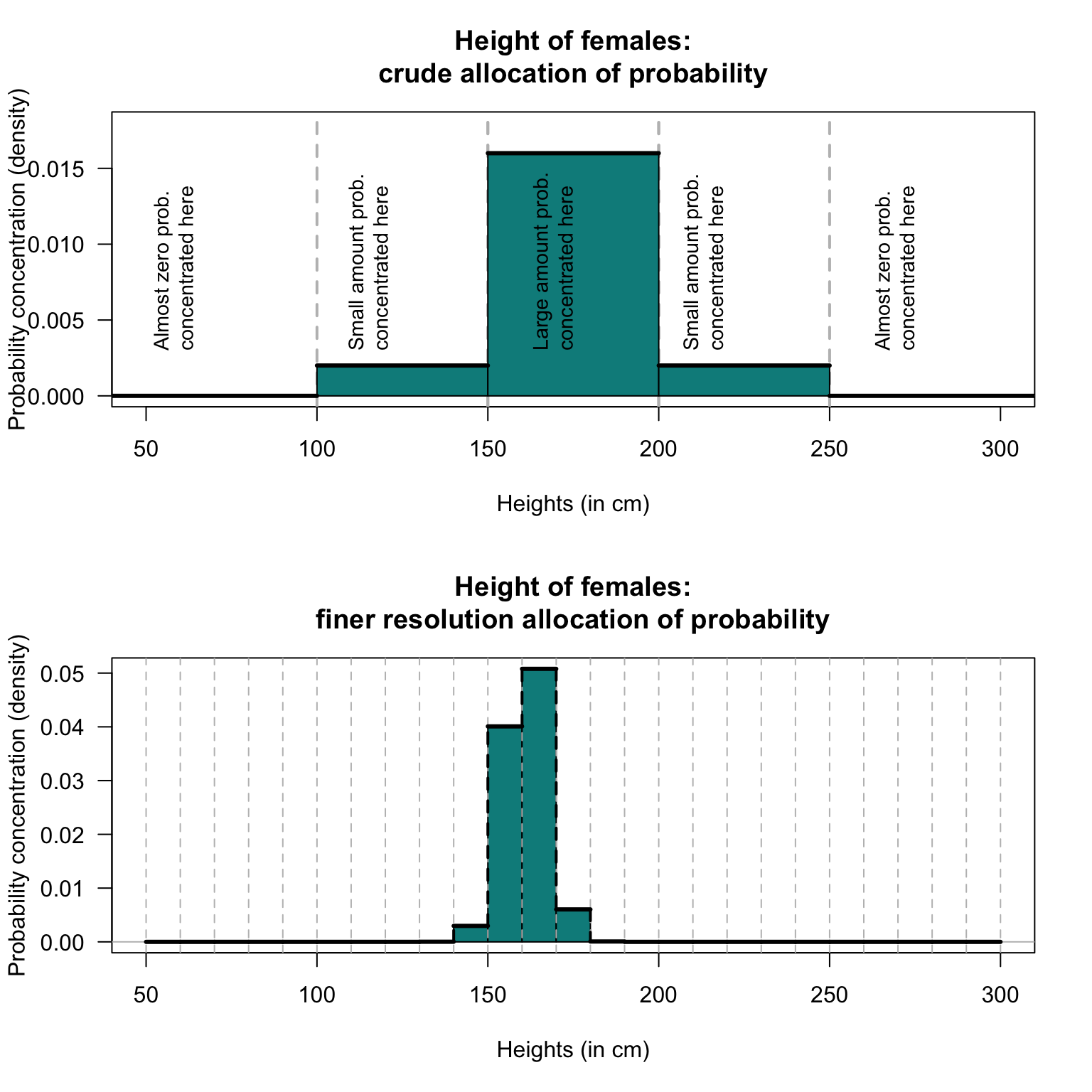
FIGURE 3.3: Allocating the concentration of probability over regions of the sample space. The shaded regions have an area of \(1\).

For a continuous sample space, intervals of the sample space represent continuous events, and areas under the curve represent probabilities for these events.

3.7.2 Probability density functions

As the intervals become smaller, the graph showing the allocation of probability become smoother (Fig. 3.4). This smooth curve, say \(f(x)\), is called a probability density function (or PDF): it shows the density (or concentration) of probability over various ranges of the sample space; for any interval \((a, b)\), the probability is \(\Pr(a < X < b) = \int_a^b f(x)\, dx\).

In discrete spaces, probabilities are summed; in continuous spaces, densities are integrated.

Definition 3.16 (Probability density function) A function \(f(x)\) defined over a sample space \(S\) is a probability density function (PDF) if

1. \(f(x) \ge 0\) for all \(x\in S\); and
2. \(\int_S f(x)\, dx = 1\).

Then \(\displaystyle \Pr(a < X < b) = \int_a^b f(x)\, dx\).

The integral over the sample space \(S\) must equal one: \[ \int_S f(x)\,dx = 1. \] The vertical axis does not represent probabilities, and often is not given.

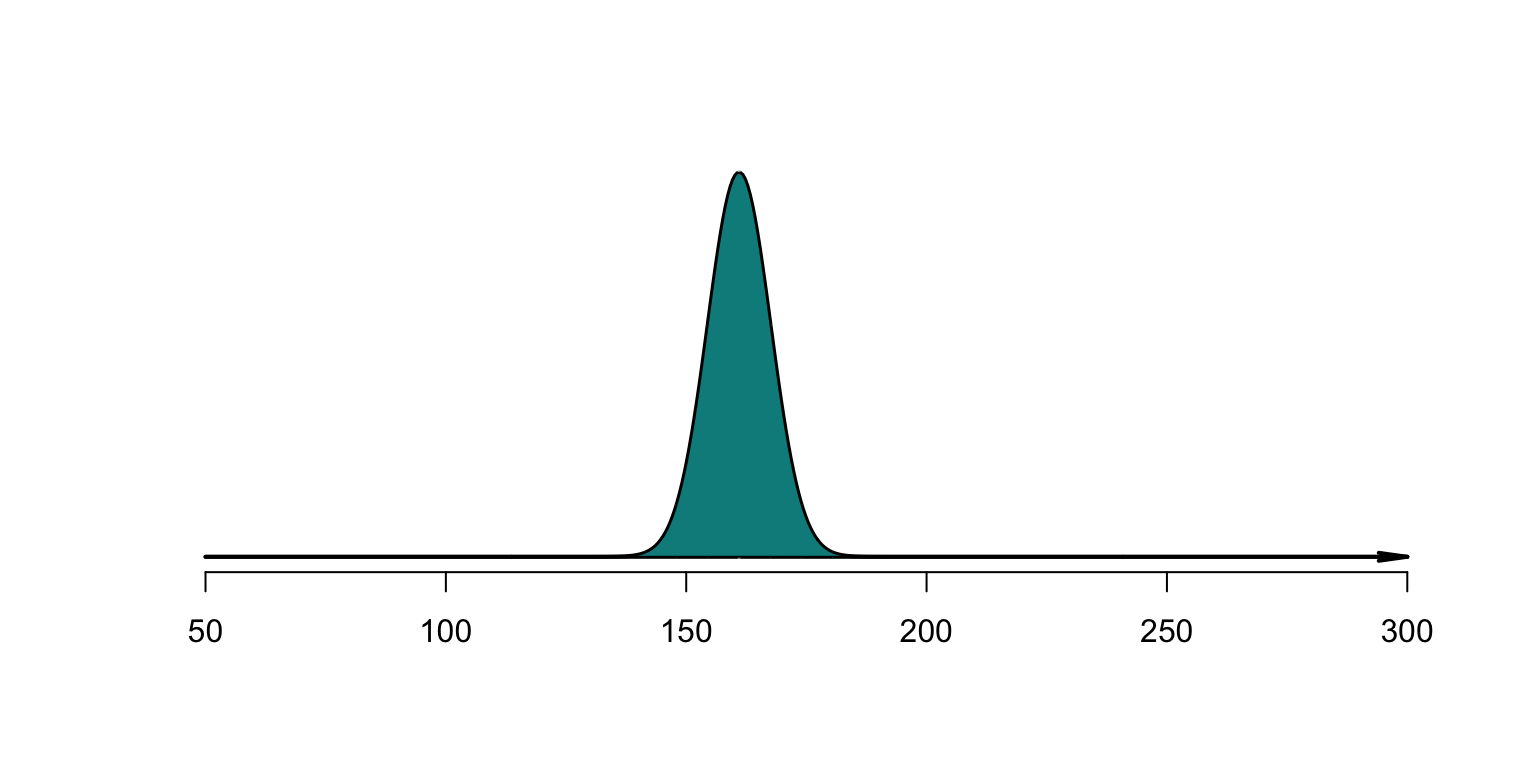
FIGURE 3.4: Smoothly allocating the concentration of probability over regions of the sample space. The shaded region has an area of \(1\).

With continuous sample spaces, the probability of observing an event \(E\) is assigned to a region (subset) of the sample space \(S\). The probability of event \(E\) is \[ \Pr(E) = \int_E f(x)\,dx. \]

For continuous random variables, probabilities are computed by integrating a probability density function \(f(x)\), which must satisfy:

1. Non-negativity: Integration over any region of the sample space must never produce a negative value, and so \(f(x) \ge 0\) for all values of \(x\).
2. Exhaustive: Over the whole sample space, the probability function must integrate to one: \[ \int_S f(x)\,dx = 1. \]
3. Additivity: The probability of the union of any non-overlapping regions is the sum of the individual regions: \[ \int_{A_1} f(x)\, dx + \int_{A_2} f(x)\, dx = \int_{A_1 \cup A_2} f(x)\, dx. \]

Using these axioms implies a probability function for some event \(A\) is defined on the continuous sample space \(S\) as \[ \Pr(X\in A) = \int_{A} f_X(x)\, dx. \]

The probability function \(f_X(x)\) does not give the probability of observing the value \(X = x\). Because the sample space has an infinite number of elements, the probability of observing any single point is zero. Instead, probabilities are computed for intervals.

This implies that \(f_X(x) > 1\) may be true for some values of \(x\), provided the total area over the sample space is one.

3.8 Assigning probability: subjective approach

‘Subjective’ probabilities are estimated after identifying the information that may influence the probability, and then evaluating and combining this information. You use this method when someone asks you about your team’s chance of winning on the weekend, for example.

A (subjective) probability may, for example, be computed using mathematical models that use the relevant information. When different people or systems identify different information as relevant, and combine them differently, different subjective probabilities eventuate.

Some examples include:

• What is the chance that an investment will return a positive yield next year? Different economists will have different subjective opinions.
• How likely is it that Auckland will have above average rainfall next year? Different people will have different subjective opinions.

Subjective probabilities can be used for discrete or continuous sample space; as always, probabilities can only be allocated to regions for continuous sample spaces.

Example 3.25 (Subjective probability) What is the likelihood of rain in Charleville (a town in western Queensland) during April? Many farmers could give a subjective estimate of the probability based on their experience and the conditions on their farm.

Using the classical approach to determine the probability is not possible. While two outcomes are possible—it will rain, or it will not rain—these are almost certainly not equally likely.

A relative frequency approach could be adopted. Data from the Bureau of Meterology, from 1942 to 2022 (81 years), shows rain fell in 71 years during April. An approximation to the probability is therefore \(71 / 81 = 0.877\), or \(87.7\)%. This approach does not take into account current climatic or weather conditions, that can change (often substantially) every year.

3.9 Using diagrams to visualise outcomes

3.9.1 Venn diagrams

Venn diagrams (see Sect. 2.6) can be useful for visualising probabilities, using regions (often circles) to represent events. Venn diagrams are useful for two events, sometimes for three, but become unworkable for more than three. Often, tables can be used to better represent situations shown in Venn diagrams (Sect. 3.9.2).

Example 3.26 (Venn diagrams) Suppose Event A has probability \(\Pr(A) = 0.4\) and Event B has \(\Pr(B) = 0.3\) on some sample space \(S\). In addition, \(\Pr(A\cap B) = 0.1\). A Venn diagram (Fig. 3.5) shows the two events in the sample space. The intersection (with probability \(0.1\)) includes elements from both Event \(A\) and Event \(B\) (and so the circles overlap).

We can see, for example, that \(\Pr(A\setminus B) = 0.3\), and \(\Pr(A\cup B) = 0.6\).

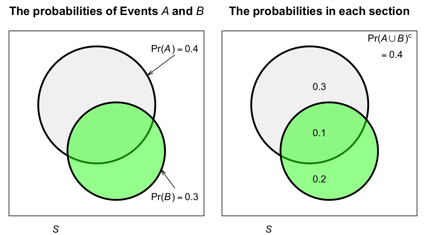
FIGURE 3.5: A Venn diagram for a simple situation with two events. The rectangle represents the sample space \(S\); the light circle represents Event \(A\) and the darker circle represents Event \(B\). Left: the two events. Right: the probabilities for each section of the sample space.

3.9.2 Tables of probability

With two variables of interest, probability tables may be a convenient way of summarizing the information. A probability represents the whole sample space, and shows how the sample space is divided between two events.

Example 3.27 (Probability tables) The information in Example 3.26 can be compiled into a two-way table (Table 3.5): Events \(A\) and \(A^c\) are shown in the columns, and Events \(B\) and \(B^c\) are shown in the rows.

TABLE 3.5: The probabilities in a two-way table for two events.

	A	Not A	Total
B	0.1	0.2	0.3
Not B	0.3	0.4	0.7
Total	0.4	0.6	1.0

3.9.3 Tree diagrams

Tree diagrams are useful when a random process can be seen, or thought of, as occurring in distinct steps or stages. The probabilities in the second step may depend on what happens on the first step. The same ideas extend to more than two steps.

Example 3.28 (Tree diagrams) A small business sells from a physical shop and also online.

Suppose the probability that a customer makes a purchase using the online store is \(0.35\); then, the probability that the customer requests a refund is \(0.30\). However, if a customer makes a purchase using the physical store, the probability that the customer requests a refund is \(0.05\). That is, most customers make purchases at the physical store, and these customers are less likely to request a refund compared to online customers.

The two events of interest are: \[\begin{align*} P&: \text{The customer makes a purchase from the physical store; and}\\ R&: \text{The customer requests a refund.} \end{align*}\] Using this notation, \(\Pr(P) = 0.65\), and so \(\Pr(P^c) = 0.35\) is the probability that a customer makes a purchase in a physical store. The value of \(\Pr(R)\) (and hence \(\Pr(R)\)) depends on whether the purchase was made online or in-store.

The situation can be considered as having two stages. Stage 1 is where the purchase was made (online, or in a physical store). Stage 2 is whether the customer requests a refund. The tree diagram for the situation is shown in Fig. 3.6. The probabilities in Stage 2 are different, depending on where the purchase was made.

To understand how to use tree diagrams requires a study of conditional probability, which we do next.

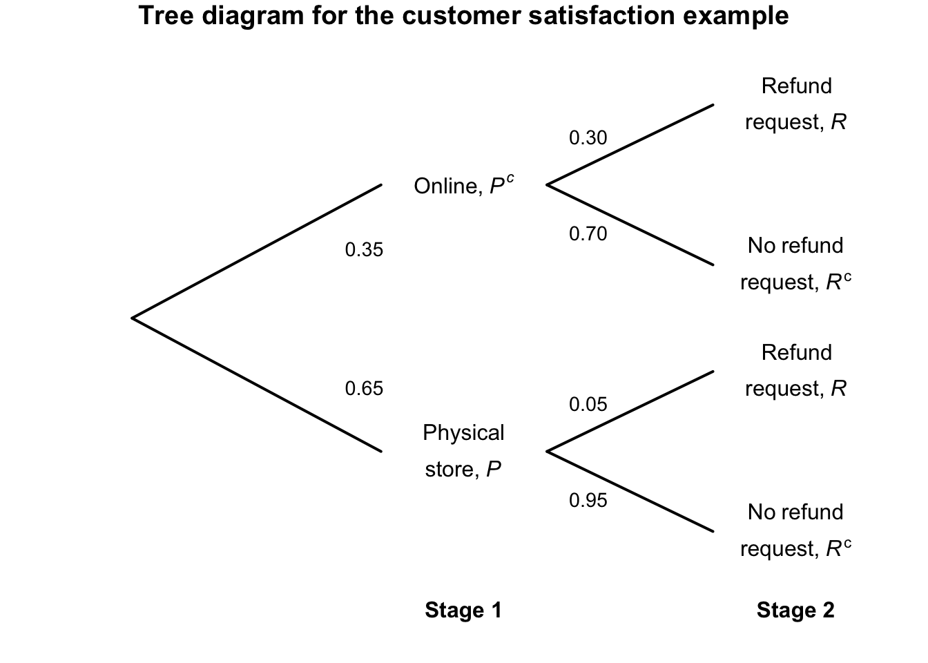
FIGURE 3.6: Tree diagram for the customer-satisfaction example.

3.10 Conditional probability and independent events

3.10.1 Conditional probability

The tree diagram in Example 3.28 is an example of conditional probability: the probability of requesting a refund is conditional on (or depends on) whether the customer made an online or physical-store purchase.

In Example 3.28, \(\Pr(R) = 0.05\) if event \(P\) has occurred; we write \(\Pr(R \mid P ) = 0.05\), which we read as ‘The probability that Event \(R\) occurs given that Event \(P\) has occurred’. \(\Pr(R \mid P)\) is a conditional probability.

We see also that \(\Pr(R) = 0.30\) if event \(P\) has not occurred; we write \(\Pr(R \mid P^c ) = 0.30\), which we read as ‘The probability that Event \(R\) occurs given that Event \(P\) has not occurred’. \(\Pr(R \mid P^c )\) is also a conditional probability.

More generally, assume that a sample space \(S\) for the random process has been constructed, an event \(A\) has been identified, and its probability \(\Pr(A)\) has been determined. We then receive additional information that some event \(B\) has occurred. Possibly, this new information can change the value of \(\Pr(A)\).

The probability that \(A\) will occur may depend on whether the information provided by event \(B\). We call this probability the conditional probability of \(A\) given \(B\), denoted by \(\Pr(A \mid B)\).

Example 3.29 (Conditional probability) Suppose I roll a die. Define event \(A\) as ‘rolling a 6’. Then, you would compute \(\Pr(A) = 1/6\) (using the classical approach; Sect. 3.5.1).

However, suppose I provide you with extra information: the number that I rolled is an even number. Define Event \(B\) as the event ‘the number rolled is even’.

With this extra information, only three numbers could possibly have been rolled; the reduced sample space is \[ S^* = \{2, 4, 6 \}. \] All of these three outcomes are equally likely. However, the probability that the number is a six is now \(\Pr(A\mid B) = 1/3\).

Knowing the extra information, that Event \(B\) had occurred, changed the calculation of \(\Pr(A)\).

Example 3.30 (Planes) Consider these two events: \[\begin{align*} D:&\quad \text{A person dies};\\ F:&\quad \text{A person falls from an airborne plane with no parachute}. \end{align*}\] Consider the probability \(\Pr(D \mid F)\). If you are told that someone falls out of an airborne plane with no parachute, the probability that they die is very high.

Then, consider the probability \(\Pr(F\mid D)\). If you are told that some has died, the cause is very unlikely to be a fall from an airborne plane without a parachute.

Thus, the first probability is very close to one, and the second is very close to zero.

Two methods exist for computing conditional probability: first principles, or a formal definition of \(\Pr(A \mid B)\). Using first principles, consider the original sample space \(S\): remove the sample points inconsistent with the new information that \(B\) has provided; form a new sample space, say \(S^*\); then recompute the probability of Event \(A\) relative to \(S^*\). \(S^*\) is called the reduced sample space.

This method is appropriate when the number of outcomes is relatively small. The following formal definition applies more generally.

Definition 3.17 (Conditional probability) Let \(A\) and \(B\) be events in \(S\) with \(\Pr(B) > 0\). Then \[ \Pr(A \mid B) = \frac{\Pr(A\cap B)}{\Pr(B)}. \]

The definition automatically takes care of the sample space reduction.

Example 3.31 (Rainfall) Consider again the rainfall at Charleville in April (Example 3.25). Define \(W\) as the event ‘receiving more than \(30\) mm in April’, and \(R\) as the event ‘receiving any rainfall in April’. Event \(W\) occurs 24 times in the 81 years of data, while Event \(R\) occurs 71 times in \(81\) years.

Using the relative frequency approach with the Bureau of Meteorology data, the probability of obtaining more than \(30\) mm in April is: \[ \Pr(W) = \frac{24}{81} = 0.296. \] However, the conditional probability of receiving more than \(30\) mm, given that rainfall was recorded, is: \[ \Pr(W \mid R) = \frac{\Pr(W \cap R)}{\Pr(R)} = \frac{\Pr(W)}{\Pr(R)} = \frac{0.2963}{0.8765} = 0.338. \] If we know rain has fallen, the probability that the amount was greater than \(30\) mm is 0.338. Without this prior knowledge, the probability is \(0.296\).

3.10.2 General multiplication rule

A consequence of Def. 3.17 is the following theorem.

Theorem 3.1 (General multiplication rule for probabilities) For any events \(A\) and \(B\), the probability of the intersection of \(A\) and \(B\) is \[\begin{align*} \Pr(A\cap B) &= \Pr(A)\cdot \Pr(B \mid A)\\ &= \Pr(B)\cdot \Pr(A \mid B). \end{align*}\]

This rule can be generalised to any number of events. For example, for three events \(A\), \(B\) and \(C\), \[ \Pr(A\cap B\cap C) = \Pr(A)\cdot\Pr(B\mid A)\cdot\Pr(C\mid A\cap B). \]

Example 3.32 (General multiplication rule) Consider again the probabilities in Example 3.28. We have \(\Pr(P) = 0.05\); then: \[\begin{align*} \Pr(R \mid P) &= 0.05\quad\text{and so}\quad \Pr(R^c \mid P) = 0.95;\\ \Pr(R \mid P^c) &= 0.30\quad\text{and so}\quad \Pr(R^c \mid P^c) = 0.70. \end{align*}\] Using the general multiplication rule, \[\begin{align*} \Pr(R \cap P) &= \Pr(R \mid P) \times \Pr(P) = 0.05\times 0.65 = 0.0325;\\ \Pr(R^c \cap P) &= \Pr(R^c \mid P) \times \Pr(P) = 0.95\times 0.65 = 0.6275;\\ \Pr(R \cap P^c) &= \Pr(R \mid P^c) \times \Pr(P^c) = 0.30\times 0.35 = 0.105;\\ \Pr(R^c \cap P^c) &= \Pr(R^c \mid P^c) \times \Pr(P^c) = 0.70\times 0.35 = 0.245. \end{align*}\] These four probabilities represent the ‘final destinations’ in the tree diagram, which we can now add to (Fig. 3.7). Notice that these probabilities on the right add to one, as they represent the entire sample space: every customer is represented on one of the four branches.

We can also determine the probability that a customer requests a refund: \[ \Pr(R) = \Pr(R \cap P) + \Pr(R \cap P^c) = 0.0325 + 0.105 = 0.1375. \] We can then determine the probability that a customer was an online customer, given that a refund was requested \[ \Pr(P\mid R) = \frac{\Pr(P\cap R)}{\Pr(R)} = \frac{0.105}{0.1375} = 0.7636\dots. \] If a refund is requested, the probability the customer was an online shopper is about \(0.76\).

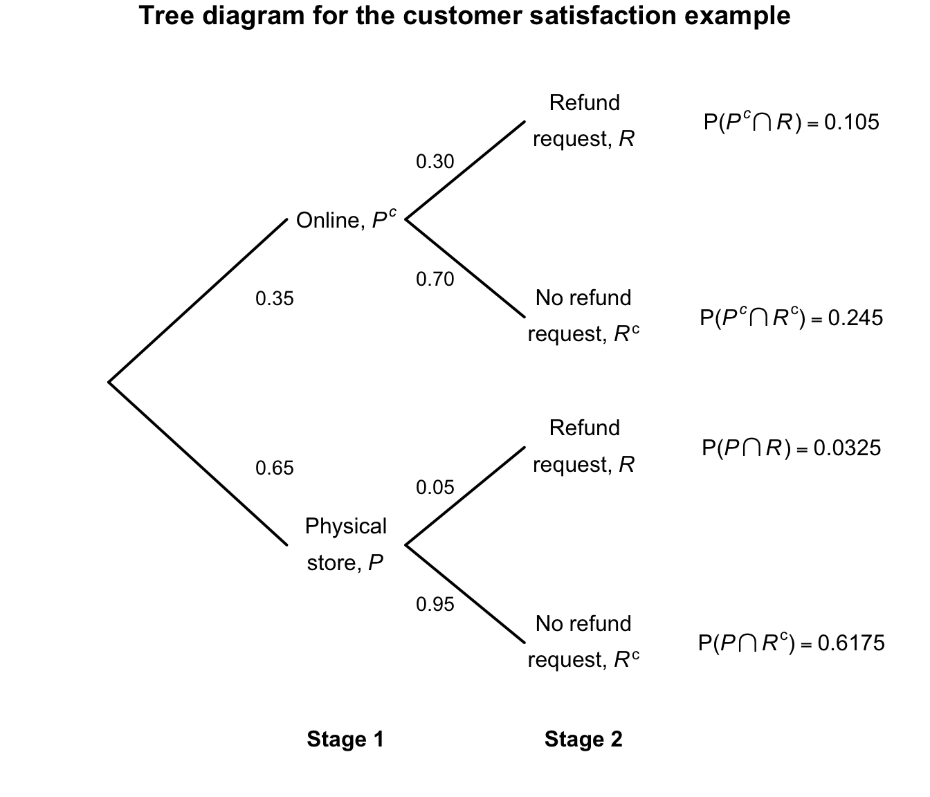
FIGURE 3.7: Tree diagram for the customer-satisfaction example, adding the probabilities of the four outcomes.

The tree diagram in Example 3.28 is an example of using conditional probability: the probability of requesting a refund is conditional on (or depends on) whether the customer made an online or in-store purchase.

3.10.3 Independent events

The important idea of independent events can now be defined.

Definition 3.18 (Independence) Two events \(A\) and \(B\) are independent events if and only if \[ \Pr(A\cap B) = \Pr(A)\Pr(B). \] Otherwise the events not independent (or, less commonly, dependent).

Provided \(\Pr(B) > 0\), Defs. 3.17 and 3.18 show that \(A\) and \(B\) are independent if, and only if, \(\Pr(A \mid B) = \Pr(A)\). This statement of independence makes sense: \(\Pr(A \mid B)\) is the probability of \(A\) occurring if \(B\) has already occurred, while \(\Pr(A)\) is the probability that \(A\) occurs without any knowledge of whether \(B\) has occurred or not. If these are equal, then \(B\) occurring has made no difference to the probability that \(A\) occurs, which is what independence means.

Example 3.33 (Independence) Soud et al. (2009) discusses the response of students to a mumps outbreaks in Kansas in 2006. Students were asked to isolate; Table 3.6 shows the behaviour of male and female student in the studied sample.

For females, the probability of complying with the isolation request is: \[ \Pr(\text{Compiled} \mid \text{Females}) = 63/84 = 0.75. \] For males, the probability of complying with the isolation request is \[ \Pr(\text{Compiled} \mid \text{Males}) = 36/48 = 0.75. \]

Whether we look at only females or only males, the probability of selecting a student in the sample that complied with the isolation request is the same: \(0.75\). Also, the non-conditional probability that a student isolated (ignoring their sex) is: \[ \Pr(\text{Student isolated}) = \frac{99}{132} = 0.75. \] In Example 3.33, the probability of males isolating was the same as the probability of females isolating. In the sample, the sex of the student is independent of whether they isolate. That is, whether we look at females or males, the probability that they isolated is the same.

TABLE 3.6: Students response to isolation request at a Kansas university.

	Complied with isolation	Did not comply with isolation	TOTAL
Females	63	21	84
Males	36	12	48

The idea of independence can be generalised to more than two events. For three events, the following definition of mutual independence applies, which naturally extends to any number of events.

Definition 3.19 (Mutual independence) Three events \(A\), \(B\) and \(C\) are mutually independent if, and only if, all of these are true: \[\begin{align*} \Pr(A\cap B) & = \Pr(A)\cdot \Pr(B).\\ \Pr(A\cap C) & = \Pr(A)\cdot \Pr(C).\\ \Pr(B\cap C) & = \Pr(B)\cdot \Pr(C).\\ \Pr(A\cap B\cap C) & = \Pr(A)\cdot \Pr(B)\cdot \Pr(C). \end{align*}\]

Three events can be pairwise independent in the sense of Def. 3.18, but not be mutually independent.

Example 3.34 (Pairwise independence) Suppose a coin is tossed three times, so that the sample space has \(2^3 = 8\) events. The following three events are defined: \[\begin{align*} A:&\ \text{First two tosses the same} = \{HHT, HHH, TTH, TTT\};\\ B:&\ \text{Last two tosses the same} = \{HHH, THH, HTT, TTT\};\\ C:&\ \text{First and last tosses the same} = \{HHH, HTH, THT, TTT \}. \end{align*}\] Thus, we see that \(\Pr(A) = \Pr(B) = \Pr(C) = 4/8 = 1/2\).

Furthermore, each pair of events is pairwise independent; for example: \[ \Pr(A\cap B) = \Pr(HHH, TTT) = 2/8 = 1/4, \] which is the same as \(\Pr(A)\times\Pr(B) = 1/4\).

Similarly, \(\Pr(A\cap C) = \Pr(A)\times\Pr(C) = 1/45\) and \(\Pr(B\cap C) = \Pr(B)\times\Pr(C) = 1/4\). This shows that each pair of events is independent.

However, \(\Pr(A\cap B\cap C) = \Pr(TTT, HHH) = 2/8 = 1/4\), but \[ \Pr(A)\times \Pr(B)\times \Pr(C) = \left(\frac{1}{2}\right)^3 = \frac{1}{8}. \] Since \(\Pr(A)\times \Pr(B)\times \Pr(C) \ne \Pr(A\cap B\cap C)\), the three events are not mutually independent.

Knowing any two constraints forces the third outcome. For example, if we know that \(A = \{T, T\}\) and independently that \(B = \{T, T\}\), then \(C\) must be \(\{T, T\}\). So pairwise independence holds, but full independence fails.

The following theorem concerning independent events is sometimes useful.

Theorem 3.2 (Independent events) If \(A\) and \(B\) are independent events, then

• \(A\) and \(B^c\) are independent.
• \(A^c\) and \(B\) are independent.
• \(A^c\) and \(B^c\) are independent.

Proof. Exercise.

3.10.4 Independent and mutually exclusive events

Mutually exclusive events (Def. 3.7) and independent events (Def. 3.18) sometimes get confused.

The simple events defined by the outcomes in a sample space are mutually exclusive, since only one can occur in any realisation of the random process. Mutually exclusive events have no common outcomes: for example, both passing and failing this course is not possible in the one semester. Obtaining one outcome excludes the possibility of the other outcome occurring… so whether one occurs depends on whether the other has occurred.

In contrast, if two events are independent, then whether or not one occurs does not affect the chance of the other happening. If event \(A\) can occur, then \(B\) happening will not influence the chance of \(A\) happening if they are independent, so it does not exclude the possibility of the other occurring.

Confusion between mutual exclusiveness and independence arises sometimes because the sample space is not clearly identified.

To demonstrate the difference, consider a random process involving tossing two coins at the same time. The sample space is \[ S_2 = \{HH, HT, TH, TT\} \] and these outcomes are mutually exclusive, each with probability \(1/4\) (using the classical approach). For example, \(\Pr( HH) = 1/4\).

An alternative view of this random process is to think of repeating the process of tossing a coin once. For one toss of a coin, the sample space \[ S_1 = \{ H, T \} \] and \(\Pr(H) = 1/2\) is the probability of getting a head on the first toss. This is also the probability of getting a head on the second toss.

The events ‘getting a head on the first toss’ and ‘getting a head on the second toss’ are not mutually exclusive, because both events can occur together: the event \((HH)\) is an outcome in \(S_2\). Whether or not the outcomes \((HH)\) occurred simultaneously (because the two coins were tossed at the one time) or sequentially (in that one coin was tossed twice) is irrelevant.

Our interest is in the joint outcomes from two tosses. The event ‘getting a head on the “first” toss’ is: \[ E_1 = \{ HH, HT \} \] and ‘getting a head on the “second” toss’ is \[ E_2 = \{ HH, TH \}, \] where \(E_1\) and \(E_2\) are events defined on \(S_2\). This makes it clear that Events \(E_1\) and \(E_2\) are not mutually exclusive because \(E_1\cap E_2 \ne \varnothing\).

The two events \(E_1\) and \(E_2\) are independent because, whether or not a head occurs on one of the tosses, the probability of a head occurring on the other is still \(1/2\). Seeing that the events are independent provides another way of calculating the probability of the two heads occurring ‘together’: \(1/2\times 1/2 = 1/4\), since the probabilities of independent events can be multiplied

Example 3.35 (Mendell's peas) Mendel (1886) conducted famous experiments in genetics. In one study, Mendel crossed a pure line of round yellow peas with a pure line of wrinkled green peas. Table 3.7 shows what happened in the second generation for a sample of peas. For example, \(\Pr(\text{round peas}) = 0.7608\). Biologically, about \(75\)% of peas are expected to be round; the data appear reasonably sound in this respect.

Is the type of pea (rounded or wrinkled) independent of the colour? That is, if the pea is rounded, does it impact the colour of the pea?

Independence can be evaluated using the formula is \(\Pr(\text{round} \mid \text{yellow}) = \Pr(\text{round})\). In other words, the fact that the pea is yellow does not affect that probability that the pea is rounded. From Table 3.7: \[\begin{align*} \Pr(\text{rounded}) &= 0.5665 + 0.1942 = 0.7608,\\ \Pr(\text{round} \mid \text{yellow}) &= 0.5665/(0.5665 + 0.1817) = 0.757. \end{align*}\]

These two probabilities are very close. The data in the table are just a sample (from the population of all peas), so assuming the colour and shape of the peas are independent is reasonable.

TABLE 3.7: The proportion of peas in the second generation results from Mendel’s experiment, crossing a pure line of round yellow peas with a pure line of wrinkled green peas.

	Yellow	Green
Rounded	0.5665	0.1942
Wrinkled	0.1817	0.0576

3.10.5 Partitioning the sample space

The concepts introduced in this section allow us to determine the probability of an event using the event-partitioning approach, which we now discuss.

Definition 3.20 (Partitioning) The events \(B_1, B_2, \ldots , B_k\) are said to represent a partition of the sample space \(S\) if

1. the events are mutually exclusive: \(B_i \cap B_j = \varnothing\) for all \(i \neq j\).
2. the events are exhaustive: \(B_1 \cup B_2 \cup \ldots \cup B_k = S\).
3. the events have a non-zero probability of occurring: \(\Pr(B_i) > 0\) for all \(i\).

The implication is that when the random process is performed, exactly one and only one of the events \(B_i\) (\(i = 1, \ldots, k)\) occurs. We use this concept in the following theorem.

Theorem 3.3 (Law of total probability) Let \(A\) be an event in \(S\) and \(\{B_1, B_2, \ldots , B_k\}\) a partition of \(S\). Then \[\begin{align*} \Pr(A) &= \Pr(A \mid B_1) \cdot \Pr(B_1) + \Pr(A \mid B_2) \cdot \Pr(B_2) + \ldots \\ & \qquad {} + \Pr(A \mid B_k) \cdot \Pr(B_k). \end{align*}\]

Proof. The proof follows from writing \(A = (A\cap B_1) \cup (A\cap B_2) \cup \ldots \cup (A\cap B_k)\), where the events on the RHS are mutually exclusive. The third axiom of probability together with the multiplication rule yield the result.

Seeing the partitioning visually is helpful. Suppose a sample space \(S\) is divided into six partitions \(B_1\), \(B_2\), \(B_3\), \(B_4\), \(B_5\) and \(B_6\), as shown in Fig. 3.8.

Event \(A\) overlaps with each of the events \(B_j\) for \(j = 1, \dots, 6\). The overlaps of event \(A\) with each partition \(B_j\) are the intersections \(\Pr(A\cap B_j)\). Event \(A\) is the sum of all these intersections: \[ \Pr(A) = \sum_{J = 1}^6 \Pr(A\cap B_j) = \sum_{J = 1}^6 \Pr(A\mid B_j)\cdot \Pr(B_k). \] For example, \(\Pr(A\mid B_6) = 1\) from Fig. 3.8).

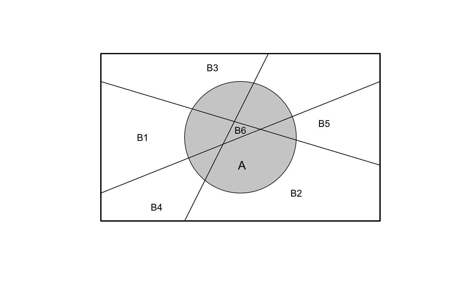
FIGURE 3.8: Partitioning the sample space into six parts (\(B_1\) to \(B_6\)), and event \(A\).

Example 3.36 (Law of total probability) Consider event \(A\): ‘rolling an even number on a die’, and also define the events \[ B_i:\quad\text{The number $i$ is rolled on a die} \] where \(i = 1, 2, \dots 6\). The Events \(B_i\) represent a partition of the sample space, as the Events \(B_i\) are mutually exclusive, exhaustive and all have non-zero probability of occurring.

Then, using the Law of total probability (Sect. 3.3): \[\begin{align*} \Pr(A) &= \Pr(A \mid B_1)\times \Pr(B_1)\quad + \quad\Pr(A \mid B_2)\times \Pr(B_2) \quad+ {}\\ &\quad \Pr(A \mid B_3)\times \Pr(B_3)\quad + \quad\Pr(A\mid B_4)\times \Pr(B_4) \quad+ {} \\ &\quad \Pr(A \mid B_5)\times \Pr(B_5)\quad + \quad\Pr(A\mid B_6)\times \Pr(B_6)\\ &= \left(0\times \frac{1}{6}\right) + \left(1\times \frac{1}{6}\right) + {} \\ &\quad \left(0\times \frac{1}{6}\right) + \left(1\times \frac{1}{6}\right) + {}\\ &\quad \left(0\times \frac{1}{6}\right) + \left(1\times \frac{1}{6}\right) = \frac{1}{2}. \end{align*}\] This the same answer obtained using the classical approach.

3.10.6 Bayes’ theorem

If an event is known to have occurred (i.e., has non-zero probability), and the sample space is partitioned, a result known as Bayes’ theorem enables us to determine the probabilities associated with each of the partitioned events.

Theorem 3.4 (Bayes' theorem) Let \(A\) be an event in \(S\) such that \(\Pr(A) > 0\), and \(\{ B_1, B_2, \ldots , B_k\}\) is a partition of \(S\). Then \[ \Pr(B_i \mid A) = \frac{\Pr(B_i) \cdot \Pr(A \mid B_i)} {\displaystyle \sum_{j = 1}^k \Pr(B_j)\cdot\Pr(A \mid B_j)} \] for \(i = 1, 2, \dots, k\).

Proof. This is a direct application of Def. 3.17, the multiplication rule and Theorem 3.3.

Notice that the right-side includes conditional probabilities of the form \(\Pr(A\mid B_i)\), while the left-side contains the probability \(\Pr(B_i\mid A)\). In effect, the theorem takes a conditional probability of the form \(\Pr(A\mid B_i)\) and can ‘reverse’ the conditioning. We saw an example of doing this in Example 3.32.

Bayes’ theorem has many uses, as it uses conditional probabilities that are easy to find or estimate (e.g., \(\Pr(A\mid B_j)\)) to compute a conditional probability that is not easy to find or estimate (e.g., \(\Pr(B_j\mid A)\)). The theorem is the basis of a branch of statistics known as Bayesian statistics which involves using pre-existing evidence in drawing conclusions from data.

Example 3.37 (Breast cancer) The success of mammograms for detecting breast cancer has been well documented (White, Urban, and Taylor 1993). Mammograms are generally conducted on women over \(40\), though breast cancer does rarely occur in women under \(40\) also.

We can define two events of interest: \[\begin{align*} C:&\quad \text{The woman has breast cancer; and}\\ D:&\quad \text{The mammogram returns a positive test result.} \end{align*}\] As with many diagnostic tools, a mammogram is not perfect. Sensitivity and specificity are used to describe the accuracy of a test:

• Sensitivity is the probability of a true positive test result: the probability of a positive test result for people with the disease. This is written as \(\Pr(D \mid C)\).
• Specificity is the probability of a true negative test result: the probability of a negative test for people without the disease. This is written as \(\Pr(D^c \mid C^c)\).

Clearly, we would like both these probabilities to be a high as possible. For mammograms (Houssami et al. 2003), the sensitivity is estimated as about \(0.75\) and the specificity as about \(0.90\).

We can write:

• \(\Pr(D \mid C ) = 0.75\) (and so \(\Pr(D^c \mid C) = 0.25\));
• \(\Pr(D^c \mid C^c) = 0.90\) (and so \(\Pr(D \mid C^c) = 0.10\)).

Furthermore, about \(2\)% of women under \(40\) will get breast cancer (Houssami et al. 2003); that is, \(\Pr(C) = 0.02\) (and hence \(\Pr(C^c) = 0.98\)). For this study, the probabilities like as \(\Pr(D\mid C)\) are easy to find: women who are known to have breast cancer have a mammogram, and we record whether the mammogram result is positive or negative.

But consider a woman under \(40\) who gets a mammogram. When the results are returned, her interest is whether they have breast cancer, given the test results; for example \(\Pr(C \mid D)\). In other words: if the test returns a positive result, what is the probability that she actually has breast cancer? That is, we would like to take probabilities like \(\Pr(D\mid C)\), that can be found easily, and determine \(\Pr(C \mid D)\), which is of interest in practice. Using Bayes’ Theorem: \[\begin{align*} \Pr(C \mid D) &= \frac{\Pr(C) \times \Pr(D \mid C)} {\Pr(C)\times \Pr(D \mid C) + \Pr(C^c)\times \Pr(D \mid C^c) }\\ &= \frac{0.02 \times 0.75} {(0.02\times 0.75) + (0.98\times 0.10)}\\ &= \frac{0.015}{0.015 + 0.098} = 0.1327. \end{align*}\] Consider what this means. If a mammogram returns a positive test (for a woman under \(40\)), the probability that the woman really has breast cancer is only about \(6\)%… This partly explains why mammograms for women under \(40\) are not commonplace: almost all women who return a positive test result actually do not have breast cancer.

The reason for this surprising result is explained in Example 3.38.

Example 3.38 (Breast cancer) Consider using a tree diagram to describe the breast cancer information from Example 3.37 (Fig. 3.9). By following each ‘branch’ of the tree, we can compute, for example: \[ \Pr(C \cap D) = \Pr(C)\times \Pr(D\mid C) = 0.02 \times 0.75 = 0.015; \] that is, the probability that a woman has a positive test and breast cancer is about \(0.015\). But compare: \[ \Pr(C^c \cap D) = \Pr(C^c)\times \Pr(D\mid C^c) = 0.98 \times 0.10 = 0.098; \] that is, the probability that a woman has a positive test and no breast cancer (that is, a false positive) is about \(0.098\).

This explains the surprisingly result in Example 3.37: because breast cancer is so uncommon in younger women, the false positives (\(0.098\)) overwhelm the true positives (\(0.015\)).

After a positive mammogram, further tests are conducted to conform a cancer diagnosis. In younger women, almost every positive mammogram returns a negative diagnosis from further tests.

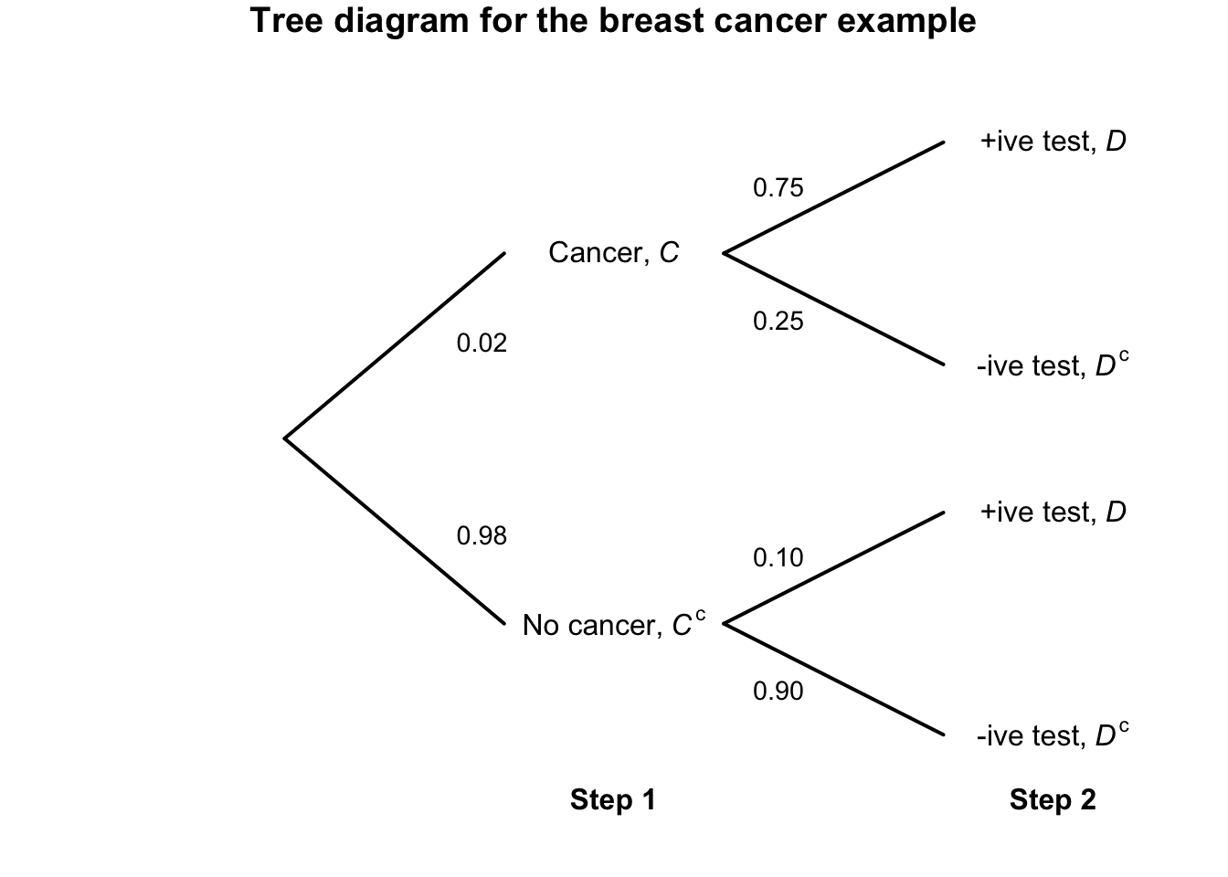
FIGURE 3.9: Tree diagram for the breast-cancer example.

Example 3.39 (Breast cancer) Consider again the breast cancer data (Example 3.37, where the events \(C\) and \(D\) were defined earlier). A Venn diagram could be constructed to show the sample space (Fig. 3.10).

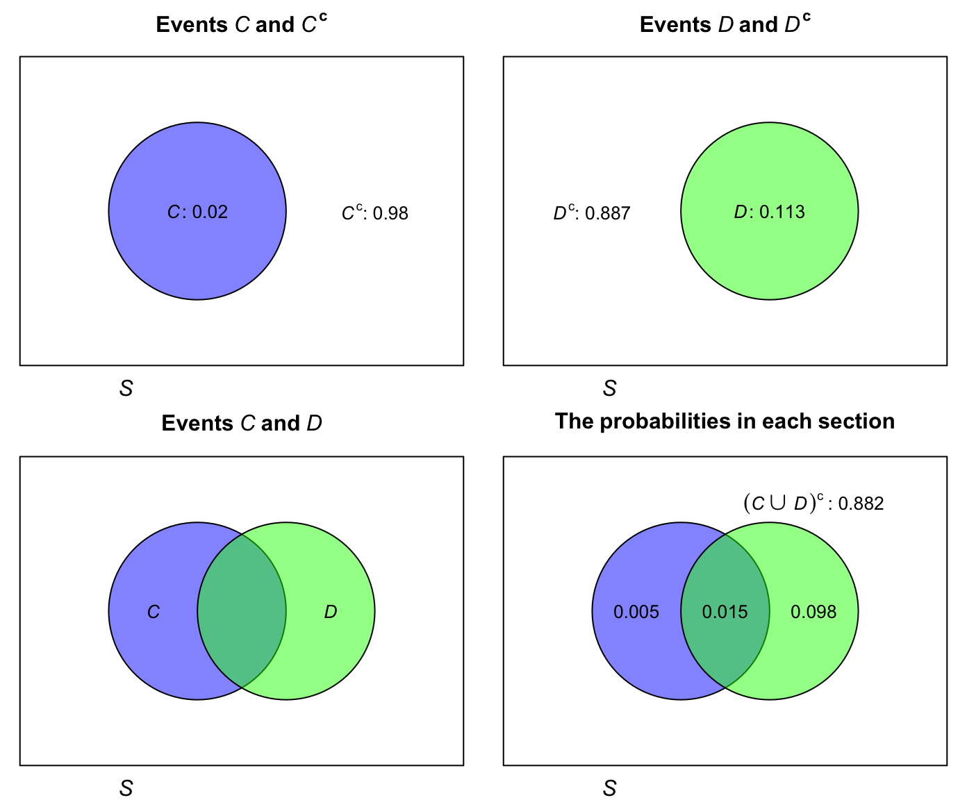
FIGURE 3.10: The Venn diagram for the breast cancer example. The rectangle in each panel represents the sample space.

3.11 Statistical computing and simulation

3.11.1 Why use computing and simulation?

Computing and working with probabilities can be hard! In many cases, using a computer, or a computer simulation, can be helpful.

Definition 3.21 (Simulation) A simulation is when a computer is used to imitate a real situation many times, so that probabilities or outcomes can be estimated.

Using a computer can be useful for many reasons when working with probabilities and statistics more generally:

1. Checking and validating results, intuition and reasoning Simulation can be used to check answers and reasoning; analytic solutions can be verified by comparing to simulation results. Simulation can confirm (not prove) counter-intuitive results (e.g., Sect. 3.11.2).
2. Demonstration of theory. Simulation can be used to visually demonstrate theory (e.g., Sect. 3.11.3). Sometimes the theory can be difficult to understand, and a simulation can bridge the gap between formulas and reality.
3. Answering tedious or complex situations. Simulation can make tedious, difficult or complex scenarios easier to understand (e.g., Sect. 3.11.4). Simulation gives quick approximations that bypass heavy combinatorial formulas. In some cases, simulation can be used for problems with no closed-form solutions.
4. Performing sensitivity analysis. Simulation allows easy tweaking or changing of parameters to see the impacts on the results (e.g., Sect. 3.11.5).

An example of each is given below. The full benefit of simulation may only be apparent in more complicated problems later in this book, once more is learnt about distribution theory.

Simulation, by definition, imitates a scenario many times. A computer is used to replicate the scenario, using random numbers (e.g., a random die roll; a random hand of cards; etc.). In general, more precise estimates of probabilities are found using a larger number of replications.

How many simulations are necessary for useful precision? No single answer exists, but since computers are fast using a large number of replications is not usually a imposition. For instance, \(5\,000\) simulations is a reasonable number for simple scenarios, but \(50\,000\) simulations may be almost as fast but provide more precision. The impact of the number of simulations is covered in more detail in Chap. 13.

Computers do not produce truly random numbers, but rather pseudo-random numbers that are generated from a random number seed. The same random number seed produces the same sequence of pseudo-random numbers. In this book, so that examples are reproducible (i.e., you will see the same results), we set the random number seed when using R (using set.seed()), so that our examples are reproducible. (Nonetheless, we call these ‘random numbers’ with the understanding that they are really pseudo-random numbers…) The R function replicate() allows an R expression to be repeated (‘replicated’) a given number of times, and often proves useful for creating simulations.

3.11.2 Simulation to confirm and validate results

Consider the breast cancer example (Example 3.37), where the probability of having breast cancer after a positive test results is quite low. This result is surprising; computer simulation can be used to confirm that this is correct.

The easiest way to simulate using the replicate() function is to first define an appropriate R function to compute the probability that a woman has breast cancer, if the test gives a positive result. Hence, first we define a suitable R function that works for one replication, then use replicate() to repeat this over many replications.

The function is defined to take four inputs:

• population_Size, which has a default value of 10000;
• cancer_Prob, which has a default value of 0.02;
• sensitivity, which has a default value of 0.75;
• specificity, which has a default value of 0.90.

The default values can be change be providing a different value to the function; if no value is given, the defaults are used. The default values are those used in Example 3.37.

The function below uses a useful ‘trick’: each patient is allocated a random number between \(0\) and \(1\) by using runif(). People with an allocated random below the value of cancer_Prob are deemed to have cancer.

P_cancer <- function(population_Size = 10000,   # Population size
                     cancer_Prob = 0.02,        # Pr(really has cancer)
                     sensitivity = 0.75,        # Pr(+ive test | has cancer)
                     specificity = 0.90) {      # Pr(-ive test | no cancer)
  
  # True cancer status: Generate a random number for each person. 
  # People with a number less than the 'threshold' have cancer.
  cancer <- runif(population_Size) < cancer_Prob
     # cancer  is a vector of TRUE and FALSE values.
     # runif(population_Size) produces that many random numbers between 0 & 1
  
  # Test results: Create a logical vector (empty for now)
  # to fill with TRUE or FALSE as appropriate.
  test_positive <- logical(population_Size)
  
  # Sensitivity: P(test positive | cancer)
  # * sum(cancer) is the number of people truly with cancer
  # * runif( sum(cancer) ) produces that many random numbers
  # * if that random number is less than 'sensitivity': positive test
  test_positive[cancer] <- runif(sum(cancer)) < sensitivity
  
  # False positive rate: 1 - specificity
  # * sum(!cancer) is the number of people truly without cancer
  # * runif( sum(!cancer) ) produces that many random numbers
  # * if that random number is less than '1-specificity': positive test
  test_positive[!cancer] <- runif(sum(!cancer)) < (1 - specificity)
  
  # Compute P(Cancer | Test positive)
  # Have to be careful: If there are no positive test results,
  # we will end up dividing by zero...
  if (sum(test_positive) == 0) return(NA)  # NA: not available
  
  mean(cancer[test_positive])
}

We can check if this function works for one replication:

P_cancer()        # This uses all the default values
#> [1] 0.120524

This probability will change each time the function is run, since it uses random numbers. Now, we can simulate over many replications:

num_Reps <- 5000    # Number of replications
set.seed(876344)    # For reproducibility

results <- replicate(num_Reps,      # Repeat this many times...
                     P_cancer())    # ... using this function

mean(results, na.rm = TRUE)     # na.rm = TRUE ignores any NAs
#> [1] 0.1328612
sd(results, na.rm = TRUE)
#> [1] 0.01004723

In Example 3.37, the probability was given as \(0.1327\), which compares favourably with this answer from simulation (which is an approximation).

The above code has three places where random numbers are used:

• to randomly allocate people to have cancer or not;
• to randomly determine which people with cancer return a positive result; and
• to randomly determine which people without cancer return a positive result.

Thus, each time the above code is run will produce different results (unless the random-number seed remains the same).

A simulation repeats the above scenario many times, over many replications each with different random numbers used. Then, the probability of interest (here, the probability of having cancer, given a positive test result) can be averaged over the many replications.

3.11.3 Simulation to demonstrate theory

The Weak Law of Large Numbers is an important statistical concept.

Definition 3.22 (Weak Law of Large Numbers) The sample proportion of a random outcome converges (in probability) to the true probability as the number of trials increases.

This can be shown by running a computer simulation, to simulate large numbers of coin tosses. First, set up the scenario:

set.seed(966141) # For repeatability

# Set the number of replications to use
Num_Tosses <- 500

Then we use the R function sample() to take a ‘sample’ of heads and tails (with replacement!) for each replication:

Tosses <- sample(x = c("H", "T"),    # Choose either "H"  or  "T"
                 size = Num_Tosses,  # Do this for each replication
                 replace = TRUE,     # H and T can be reselected 
                 prob = c(0.5, 0.5)) # Pr(Head) = Pr(Tail) = 0.5
head(Tosses)                         # Show the first few results
#> [1] "H" "T" "T" "H" "H" "H"

Notice that the probability of a Head (and Tail) is set as \(0.5\) in the simulation, to simulate tossing a coin. After each toss, the probability of obtaining a head using all the available information up to that toss was computed:

Toss_Number <- 1:Num_Tosses           # Sequence: from 1 to Num_Tosses
head(Toss_Number)                     # Show the first few values 
#> [1] 1 2 3 4 5 6

# Compute P(Heads) after each toss (cumsum()  is the 'cumulative sum')
head( cumsum(Tosses == "H") )         # head() shows the first few results
#> [1] 1 1 1 2 3 4

# Compute the proportions
Prop_Heads <- cumsum(Tosses == "H") / Toss_Number
head(Prop_Heads)                      # Show the few results
#> [1] 1.0000000 0.5000000 0.3333333 0.5000000
#> [5] 0.6000000 0.6666667

The results can be plotted (Fig. 3.11):

plot(Prop_Heads,
     main = "The proportion of heads after a given number of tosses", # Main title
     xlab = "Toss number",                        # Label on x-axis
     ylab = "Proportion of heads",                # Label on y-axis
     type = "l",           # Show a "l"ine (rather than "p"oints)
     lwd = 2,              # Make line of width '2'
     ylim = c(0, 1),       # y-axis limits
     las = 1,              # Make tick labels horizontal
     col = "cyan4")        # Line colour

# abline() draws a straight line
abline( h = 0.5,           # Draw horizontal line at y = 0.5
        col = "grey")      # Make line grey in colour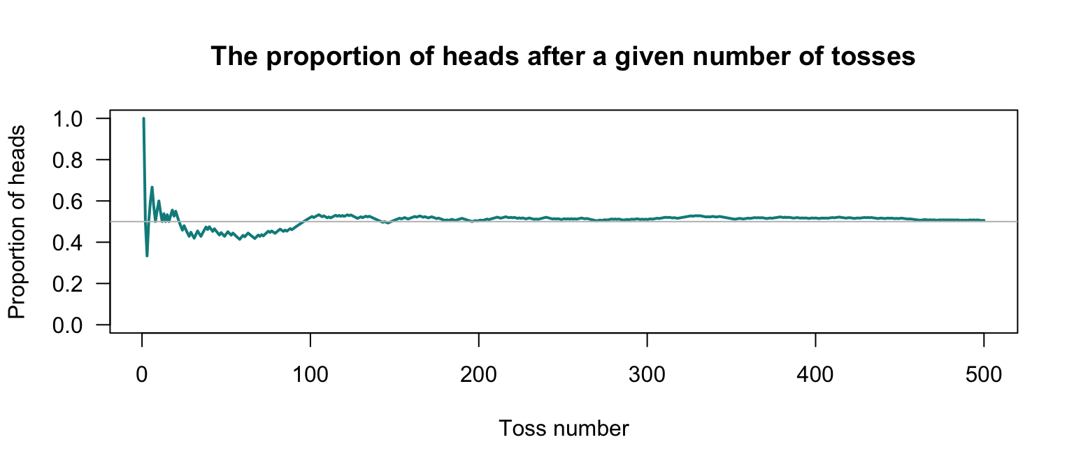

FIGURE 3.11: A simulation of tossing a fair coin \(500\) times. The probability of getting a head is computed from the data after each toss. The grey horizontal line is at \(0.5\).

For one such simulation, these running probabilities are shown in Fig. 3.11. While the result of any single toss is unpredictable, we see the Weak Law of Large Numbers in action: the sample proportion of heads approaches \(0.5\) as the number of tosses increases.

Using the empirical approach shows why probabilities are between \(0\) and \(1\) (inclusive), since the proportions \(m/n\) are always between \(0\) and \(1\) (inclusive). In this case, the sample proportion of heads converges (in probability) to the true probability of a head \(p = 0.5\) as the number of trials increases.

3.11.4 Simulation to answers tedious or complex situations

Suppose \(10\) people are invited to a party, and sit at a round table; however, two people (say, Anh and Barb) refuse to sit next to each other. What is the probability that a random seating arrangement satisfies this constraint?

This is difficult (but not impossible) to compute exactly: the number of circular permutations need to be counted, while excluding adjacent pairs. Simulation, however, could be used. The strategy is:

• Set up the simulation.
• Repeat this numerous times:
  • Create a random permutation of the seating arrangements for \(10\) people.
  • Check if Anh and Barb are ‘neighbours’ for this arrangement.
• Print the result.

Then, the process is repeated for numerous randomly-generated seating arrangements, and the proportion of acceptable seating arrangements computed.

First, set up the scenario:

set.seed(8723) # Set the random number seed, for reproducibility

num_Reps <- 5000  # Set the number of simulations

# 'Name' the 10 people by using the 'initials' of the ten people
People <- LETTERS[1:10] # The first 10 capital letters: the people
People
#>  [1] "A" "B" "C" "D" "E" "F" "G" "H" "I" "J"

Then, we create an R function to determine if Anh (who is A) and Barb (who is B) are next to each other:

# The function takes a seating arrangement as input, given as (for example) 
# "A", "J", "F", "G", "H", "I", "E", "B", "G", "J", "C", "D"
#
# It checks, for any given seating arrangement, if "A" and "B" are neighbours.

check_If_Neighbours <- function(Arrangement) {
  n <- length(Arrangement)
  
  # Allow for circular adjacency: append first element at the end
  extended <- c(Arrangement, Arrangement[1])
  
  # Compare each person with the next
  right <- extended[-1]            # right: positions 2... (n+1)
  left  <- extended[-(n + 1)]      # current: positions 1... n
  
  # Check if A next to B, or if B next to A
  are_Neighbours <- any((left == "A" & right == "B") | 
                        (left == "B" & right == "A"))
  
  return(are_Neighbours)
}

To replicate this numerous times, the R function replicate() is used; it repeatedly evaluates the given R code a specified number of times. In this case:

# Run simulation
# Summing works, because  TRUE  is treated as 1, FALSE  is treated as 0
seated_Together <- sum( replicate(num_Reps, 
                                  check_If_Neighbours( sample(People))) )
# sample(People) makes a random arrangement of the 10 people

The command first creates a random arrangement of people (i.e., sample(People)), and then checks if the given permutation of people has Anh and Barb seated as neighbours (using our function check_If_Neighbours()). This is replicated num_Reps times (using replicate()), and adds up (using sum()) how many times they are seated together. Then, the result can be printed:

# Estimated probability
prob <- seated_Together / num_Reps
cat("Prob. of an UNacceptable seating arrangement: approx. ", 
    round(prob, 4), "\n") # Round to four decimal places
#> Prob. of an UNacceptable seating arrangement: approx.  0.216

3.11.5 Simulation for sensitivity analysis

Sensitivity analysis refers to the process of checking how (and by how much) the results of a problem or model change when the inputs or assumptions are adjusted: how sensitive the results are to those inputs.

Consider again the breast cancer simulation from Sect. 3.11.2. A sensitivity analysis may consider how the final results (i.e., \(\Pr(\text{Has cancer} \mid \text{Positive test})\)) changes depending on different values of the inputs parameters.

For example, what happens if the sensitivity of the test improves, from \(0.75\) to \(0.90\)?

set.seed(8091)      # For reproducibility
num_Reps <- 5000    # Number of replications

results <- replicate(num_Reps,  
                     P_cancer(sensitivity = 0.90) )
mean(results, na.rm = TRUE)     # na.rm = TRUE ignores any NAs
#> [1] 0.1551945
sd(results, na.rm = TRUE)
#> [1] 0.01082119

While the probability has improved (i.e., got larger), it is still disturbingly low: receiving a positive test results means the probability of having breast cancer is only \(0.156\). (so not having breast cancer is still far more likely than having breast cancer).

How would the probability change if the prevalence of breast cancer was higher?

set.seed(8091)      # For reproducibility
num_Reps <- 5000    # Number of replications

results <- replicate(num_Reps,  
                     P_cancer(cancer_Prob = 0.3))    # Change the default value

mean(results, na.rm = TRUE)     # na.rm = TRUE ignores any NAs
#> [1] 0.7628346
sd(results, na.rm = TRUE)
#> [1] 0.00778957

In this scenario, the chance of actually having breast cancer after a positive test is much higher. Further sensitivity analysis confirms that the very low prevalence of breast cancer is behind the low value for \(\Pr(\text{Has cancer} \mid \text{Positive test})\)), as suggested in Example 3.38: the number of false positive tests overwhelms the number of true positive tests.

3.12 Exercises

Selected answers appear in Sect. F.2.

Exercise 3.1 Suppose \(\Pr(A) = 0.53\), \(\Pr(B) = 0.24\) and \(\Pr(A\cap B) = 0.11\).

1. Display the situation using a Venn diagram, tree diagram and a table. Which is easier in this situation?
2. Find \(\Pr(A\cup B)\).
3. Find \(\Pr(A^c\cap B)\).
4. Find \(\Pr(A^c \cup B^c)\).
5. Find \(\Pr(A \mid B)\).
6. Are events \(A\) and \(B\) independent?

Exercise 3.2 Suppose \(\Pr(A) = 0.22\), \(\Pr(B) = 0.48\) and \(\Pr(A\cap B) = 0.15\).

1. Display the situation using a Venn diagram, tree diagram and a table. Which is easier in this situation?
2. Find \(\Pr(A\cup B)\).
3. Find \(\Pr(A^c\cap B)\).
4. Find \(\Pr(A^c \cup B^c)\).
5. Find \(\Pr(A \mid B)\).
6. Are events \(A\) and \(B\) independent?

Exercise 3.3 Suppose a box contains \(100\) tickets numbered from \(1\) to \(100\) inclusive. Four tickets are drawn from the box one at a time (without replacement). Find the probability that:

1. all four numbers drawn are odd.
2. exactly two odd numbers are drawn.
3. at least two odd numbers are drawn before drawing the first even number.
4. the sum of the numbers drawn is odd.

Exercise 3.4 Suppose a box contains \(500\) tickets numbered from \(1\) to \(500\) inclusive. Six tickets are drawn from the box one at a time (without replacement). Find the probability that:

1. all six numbers drawn are odd.
2. exactly two numbers less than \(100\) are drawn.
3. at least two odd numbers are drawn before drawing the first even number.
4. all the numbers drawn are less than \(200\).

Exercise 3.5 A courier company is interested in the length of time a certain set of traffic lights is green. The lights are set so that the time between green lights in any one direction is between \(15\) and \(150\) seconds. An employee observes the lights and record the length of time between consecutive green lights.

1. What is the random variable?
2. What is the sample space?
3. Can the classical approach to probability be used to determine the probability that the time between green lights is less than \(90\) seconds? Why or why not?
4. Can the relative frequency approach be used to determine the same probability? If so, how? If not, why not?

Exercise 3.6 Street lights in a town are programmed to turn on when the light dips below a certain intensity threshold, but must be turned on by 6pm.

1. What is the random variable?
2. What is the sample space?
3. Can the classical approach to probability be used to determine the probability that the street lights are on before 5pm? Why or why not?
4. Can the relative frequency approach be used to determine the same probability? If so, how? If not, why not?

Exercise 3.7 Suppose a touring cricket squad consist of fifteen players, from which a team of eleven must be chosen for each game. Suppose a squad consists of seven batters, five bowlers, two all-rounders and one wicket-keeper.

1. Find the number of teams possible if the playing team consists of five batters, four bowlers, one all-rounder and one wicket-keeper.
2. After a game, each member of one playing team shakes hands with each member of the opposing playing team, and each member of both playing teams shakes hands with the two umpires. How many handshakes are there in total at the conclusion of a game?

Exercise 3.8 A committee comprises \(12\) people, seven of whom are male and five of whom are female. From this committee, four executive positions must be filled: President, Vice-President, Secretary and Treasurer.

1. Find the number of possible executive teams.
2. If the President must be female, how many executive teams are possible?
3. If the roles of Vice-President and the Secretary can be held by the same person, how many executive teams are possible?

Exercise 3.9 Researchers (Dexter et al. 2019) observed the behaviour of pedestrians in Brisbane, Queensland, around midday in summer. The researchers found the probability of wearing a hat was \(0.025\) for males, and \(0.060\) for females. Using this information:

1. Construct a tree diagram for the sample space.
2. Construct a table of the sample space.
3. Construct the Venn diagram of the sample space.
4. Is wearing a hat independent of gender? Explain.

Exercise 3.10 A family with six non-driving children, and two driving parents has an eight-seater vehicle.

1. In how many ways can the family be seated in the car (and legally go driving)?
2. Suppose one of the children obtains their driving licence. In how many ways can the family be seated in the car (and legally go driving) now?
3. Two of the children legally need car seats, so two car seats are fixed in the vehicle (i.e., they cannot be moved to different seats) and each child has their ‘own’ seat. If the two parents are the only drivers, in how many ways can the family be seated in the car (and legally go driving) now?

Exercise 3.11 A group of four people sit down to play Monopoly. The eight tokens are distributed randomly. In how many ways can this be done?

Exercise 3.12 A company password policy is that users must select an eight-letter password comprising lower-case letters. The company is considering each of the following changes separately:

1. Suppose the policy changes to allow eight-, nine-, or ten-letter passwords of just lower-case letters. How many passwords are possible now?
2. Suppose the policy changes to allow eight-letter passwords comprising lower-case and upper-case letters letters. How many passwords are possible now?
3. Suppose the policy changes to allow eight-letter passwords comprising lower-case, upper-case letters letters and the ten digits \(0\) to \(9\). How many passwords are possible now?
4. Suppose the policy changes to allow eight-letter passwords comprising lower-case, upper-case letters letters and the ten digits \(0\) to \(9\), and each password must have one of each category. How many passwords are possible now?

Exercise 3.13 Stirling’s approximation is \[ n!\approx {\sqrt {2\pi n}}\left({\frac {n}{e}}\right)^{n}. \]

1. Compare the values of the actual factorials with the Stirling approximation values for \(n = 1, \dots, 10\). (Use technology!)
2. Plot the relative error in Stirling’s approximation for \(n = 1, \dots, 10\), where \[ \text{relative error} = \frac{|\text{approximate value} - \text{exact value} |}{|\text{exact value}|}. \]

Exercise 3.14 Many document processors help users match brackets. For instance, the string (()) is syntactically valid, whereas ())( is not, even though both contain two opening and two closing brackets.

1. List all the ways in which two opening and two closing brackets can be written in a way that is syntactically valid.
2. How many ways can three opening and three closing brackets be written in a way that is syntactically valid? List these.
3. In general, the number of ways that \(n\) opening and \(n\) closing brackets can be written that is syntactically valid is given by the Catalan numbers \(C_n\), where: \[ C_{n} = {\frac {1}{n + 1}}\binom{2n}{n}. \] Show that an equivalent expression for \(C_n\) is \(\displaystyle C_n = {\frac {(2n)!}{(n + 1)!\,n!}}\).
4. Show that another equivalent expression for \(C_n\) is \(\displaystyle \binom{2n}{n} - \binom{2n}{n + 1}\) for \(n\geq 0\).
5. Find the first nine Catalan numbers, starting with \(C_0 = 1\).

Exercise 3.15 In a two-person game, a fair die is thrown in turn by each player. The first player to roll a wins.

1. Find the probability that the first player to throw the die wins.
2. Suppose the player who throws first is selected by the toss of a fair coin. Show that each player still has an equal chance of winning.

Exercise 3.16 To get honest answers to sensitive questions, sometimes the randomised response technique is used. For example, suppose the aim is to discover the proportion of students who have used illegal drugs in the past week.

\(N\) cards are prepared, where \(m\) have the statement ‘I have used an illegal drug in the past week’. The remaining \(N - m\) cards have the statement ‘I have not used an illegal drug in the past week’.

Each student in the sample then selects one card at random from the prepared pile of \(N\) cards, and answers ‘True’ or ‘False’ when asked the question ‘Is the statement on the selected card true or false?’ without divulging which statement is on the card. Since the interviewer does not know which card has been presented, the interviewer does not know if the person has used drugs or not from this answer.

Let \(T\) be the probability that a student answers ‘True’, and \(p\) be the probability that a student chosen at random has used an illegal drug. Assume that each student answers the question on the chosen card truthfully.

1. From an understanding of the problem, show that \[ T = (1 - p) + \frac{m}{N}(2p - 1). \]
2. Find an expression for \(p\) in terms of \(T\), \(m\) and \(N\) by rearranging the previous expression.
3. Explain what happens for \(m = 0\), \(m = N\) and \(m = N/2\), and why these make sense in the context of the question.
4. Suppose that, in a sample of 400 students, 175 answer ‘True’. Estimate \(p\) from the expression found above, given that \(N = 100\) and \(m = 25\).

Exercise 3.17 A multiple choice question contains \(m\) possible choices. There is a probability of \(p\) that a candidate chosen at random will know the correct answer. If a candidate does not know the answer, the candidate guesses and is then equally likely to select any of the \(m\) choices.

For a randomly selected candidate, what is the probability of the question being answered correctly?

Exercise 3.18 In the 2019/2020 English Premier League (EPL), at full-time the home team had won \(91\) out of \(208\) games, the away team won \(67\), and \(50\) games were drawn. (Data from: https://sports-statistics.com/sports-data/soccer-datasets/)

Define \(W\) as a win, and \(D\) as a draw.

1. Explain the difference between \(\Pr(W)\) and \(\Pr(W \mid D^c)\).
2. Compute both probabilities, and comment.

Exercise 3.19 Consider a square of size \(1\times 1\) metre. A random process consists of selecting two points at random in the square.

1. What is the sample space for the distance between the two points?
2. Suppose a grid (lines parallel to the sides) is drawn on the square such that grid lines are equally spaced \(25\) cm apart. Two points are chosen again, but must be on the intersection of the grid lines. Write some R code to generate the sample space for the distance between the two points.

Exercise 3.20 Suppose that \(30\)% of the residents of a certain suburb subscribe to a local newsletter. In addition, \(8\)% of residents belong to a local online group.

1. What percentage of residents could belong to both? Give a range of possible values.
2. Suppose \(6\)% belong to both. Compute:
   1. The probability than a random chosen newsletter subscriber is also a member of the online group.
   2. The probability than a random chosen online member is also a subscriber to the newsletter.

Exercise 3.21 The data in Table 3.8 tabulates information about school children in Queensland in 2019 (Dunn 2023).

1. What is the probability that a randomly chosen student is a First Nations student?
2. What is the probability that a randomly chosen student is in a government school?
3. Is the sex of the student approximately independent of whether the student is a First Nations student, for students in government schools?
4. Is the sex of the student approximately independent of whether the student is a First Nations student, for students in non-government schools?
5. Is whether the student is a First Nations student approximately independent of the type of school, for female students?
6. Is whether the student is a First Nations student approximately independent of the type of school, for male students?
7. Based on the above, what can you conclude from the data?

TABLE 3.8: The number of First Nations and non-First Nations students in various Queensland schools in 2019.

	Number of First Nations students	Number of non-First Nations students
Government schools
Females	2540	21219
Males	2734	22574
Non-government schools
Females	391	9496
Males	362	9963

Exercise 3.22 Two cards are randomly drawn (without replacement) from a \(52\)-card pack.

1. What is the probability the second card is an Ace?
2. What is the probability that the first card is lower in rank (Ace low) than the second?
3. What is the probability that the card ranks are in consecutive order where Ace is low or high and order is irrelevant (e.g., (Jack, Queen), (Queen, Jack), (Ace, Two) or (King, Ace))?

Exercise 3.23 An octave contains \(12\) distinct notes: seven white keys and 5 black keys on a piano.

1. How many different eight-note sequences within a single octave can be played using the white keys only?
2. How many different eight-note sequences within a single octave can be played if the white and black keys alternate (starting with either colour)?
3. How many different eight-note sequences within a single octave can be played if the white and black keys alternate and no key is played more than once?

Exercise 3.24 Find \(\Pr(A\cap B)\) if \(\Pr(A) = 0.2\), \(\Pr(B) = 0.4\), and \(\Pr(A\mid B) + \Pr(B \mid A) = 0.375\).

Exercise 3.25 Suppose the events \(A\) and \(B\) have probabilities \(\Pr(A) = 0.4\) and \(\Pr(B) = 0.3\), and \(\Pr(A\cup B) = 0.5\). Determine \(\Pr( A^c \cap B^c)\). Are \(A\) and \(B\) independent events?

Exercise 3.26 Solve \(12\times P^7_k = 7\times P^6_{k + 1}\) using:

1. algebra; and then
2. using R to search over all possible values of \(k\).

Exercise 3.27 Solve \(P^7_{r + 1} = 10 {C^7_r}\) for \(r\).

Exercise 3.28 Take a guess: how many randomly-selected individuals would you need so that the probability that at least two have the same birthday would exceed \(50\)%?

1. Show that the probability that, for a group of \(N\) randomly selected individuals, at least two have the same birthday (assuming \(365\) days in a year) can be written as \[ 1 - \left(\frac{365}{365}\right) \times \left(\frac{364}{365}\right) \times \left(\frac{363}{365}\right) \times \dots\times \left(\frac{365 - n + 1}{365}\right). \]
2. Graph the relationship for various values of \(N\), using the above form to compute the probability.
3. What assumptions are necessary? Are these reasonable?
4. Use computer simulation to confirm these results.

Exercise 3.29 Six numbers are randomly selected without replacement from the numbers \(1, 2, 3,\dots, 45\). Model this process using R to estimate the probability that there are no consecutive numbers amongst the numbers selected. (That is, no sequence like 4, 5 or 33, 34 or 21, 22, 23 appears, once the numbers are sorted smallest to largest.)

Exercise 3.30 A new cars can be purchased with options:

• Seven different paints colours are available;
• Three different trim levels are available;
• Cars can be purchased with or without a sunroof.

How many possible combinations are possible?

Exercise 3.31 Suppose number plates have three numbers, followed by two letters then another number. How many number plates are possible with this scheme?

Exercise 3.32 In some forms of poker, five cards are dealt to each player, and certain combinations then beat other combinations.

1. What is the probability that the initial five cards include exactly one pair. (This implies not getting a three of a kind or four of a kind.) Explain your reasoning.
2. What is the probability that the initial five cards includes only picture cards (Ace, King, Queen, Jack)?

Exercise 3.33 Prove that \(P^n_n = P^n_{n-1}\).

Exercise 3.34 Without using any technology, compute the value of \(\displaystyle \frac{C^{25}_8}{C^{25}_6}\).

Exercise 3.35

1. If \(A_1, A_2, \dots, A_n\) are independent events, prove that \[ \Pr(A_1 \cup A_2 \cup \dots \cup A_n) = 1 - [1 - \Pr(A_1)][1 - \Pr(A_2)] \dots [1 - \Pr(A_n)]. \]
2. Consider two events \(A\) and \(B\) such that \(\Pr(A) = r\) and \(\Pr(B) = s\) with \(r, s > 0\) and \(r + s > 1\). Prove that \[ \Pr(A \mid B) \ge 1 - \left(\frac{1 - r}{s} \right). \]

Exercise 3.36 Consider the diagram in Fig. 3.12. The point \(P\) is randomly placed within the \(1\times 1\) square \(ABCD\). What is the probability that the angle \(APB\) is greater than \(90^\circ\)?

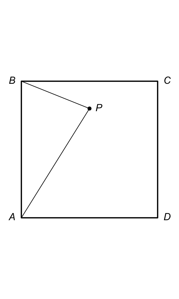
FIGURE 3.12: Point \(P\) is placed randomly in the \(1\times 1\) square \(ABCD\).

Exercise 3.37 Consider the diagram in Fig. 3.13. What is the probability that a point randomly placed within the circle (with radius \(r = 1\)) also lands within the square?

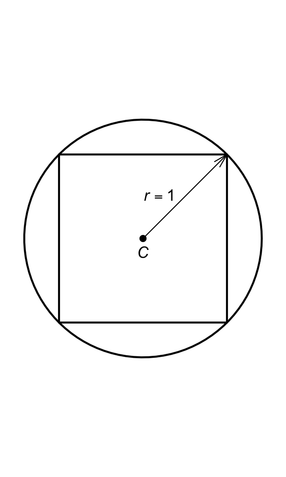
FIGURE 3.13: A random point is placed within the circle with centre \(C\) and radius \(r = 1\).

Exercise 3.38 A combination lock work by setting (for example) four digits to numbers in a specified order. Suggest a more accurate name for a ‘combination lock’.

Exercise 3.39 Consider the following dice (called Miwin’s dice);:

• Die A: The six sides are labelled: \(\qquad 2 \qquad 2 \qquad 4 \qquad 4 \qquad 9 \qquad 9\).
• Die B: The six sides are labelled: \(\qquad 1 \qquad 1 \qquad 6 \qquad 6 \qquad 8 \qquad 8\).
• Die C: The six sides are labelled: \(\qquad 3 \qquad 3 \qquad 5 \qquad 5 \qquad 7 \qquad 7\).

These dice are non-transitive that is, in the long run, Die A beats Die B, Die B beats Die C… but Die C also beats Die A.

Use a computer simulation to confirm these results by ‘rolling’ them many times, and find the probabilities of each die winning against the other two.

Exercise 3.40 Adjust the R code used in Sect. 3.11.5 so examine how the probability of running late changes as the number of booked patients increases from \(15\) up to \(25\) people.

Exercise 3.41 A game show contestant is told there is a car behind one of three doors, and a goat behind each of the other doors. The contestant is asked to select a door.

The host of the show (who knows where the car is) now opens one of the doors not selected by the contestant, and reveals a goat. The host now gives the contestant the choice of either (a) retaining the door chosen first, or (b) switching and choosing the other (unopened) door.

1. Which of the following do you think is the contestant’s best strategy?
2. Always retain the first choice.
3. Always change and select the other door.
4. Choose either unopened door at random.
5. Use a computer simulation to estimate the probabilities to determine the best strategy. Hint: remember the crucial information: the host of the show knows where the car is, and opens one of the doors not selected by the contestant, and reveals a goat.

Exercise 3.42 Suppose a specialist doctors surgery schedules a maximum of \(20\) patients per day, but history shows that each patient has a chance of not showing up (a ‘no-show’). For simplicity, assume that each patient has the same ‘no-show’ probability, and that patients operate independently. If more than \(15\) patients show up on any one day, the clinic runs late by the end of the day.

1. What is the probability the clinic runs late? Write an R function that allows for a simulation to answer the question.
2. Perform a sensitivity analysis, where the probability that each patients is a no-show varies (e.g., \(10\)%; \(15\)%; \(20\)%), to see the impact this has on the probability that the clinic runs late.
3. Perform a sensitivity analysis to see the impact on the probability of running late, if between \(18\) and \(25\) patients are booked per day.

Exercise 3.43 Consider drawing five cards at random from a fair pack; what is the probability that at least cards \(3\) are hearts?

This question is not too difficult to answer using the counting methods of Sect. 3.6; you should show that the answer is approximately \(0.0927\) using these methods.

Create an R simulation to check the answer.

---

Peter K. Dunn, Taryn Axelsen 2026: CC BY-NC-SA 4.0