7 Standard continuous distributions
On completion of this chapter, you should be able to:
- recognise the probability functions and underlying parameters of uniform, exponential, gamma, beta, and normal random variables.
- know the basic properties of the above continuous distributions.
- apply these distributions as appropriate to problem solving.
- approximate the binomial distribution by a normal distribution.
7.1 Introduction
Many of the distributions used in practice are continuous distributions. Some arise so frequently that they are given names and are studied in detail. These standard distributions act as building blocks for modelling real-world phenomena. In this chapter, the most commonly used continuous distributions are studied:
- the continuous uniform distribution models situations where every value in an interval is equally likely, which is a natural starting point for modelling complete uncertainty over a bounded range, and commonly used in simulation.
- the normal distribution is the most important distribution in all of statistics, arising naturally whenever a quantity is the result of many small independent influences; it models phenomena such as measurement errors, biological characteristics, and test scores, and underpins much of classical statistical inference.
- the exponential distribution models the time between successive random events (such as the time between customer arrivals, equipment failures, or insurance claims) and is closely linked to the Poisson distribution.
- the gamma distribution generalises the exponential to model the time until a fixed number of events occur, and is widely used in insurance, hydrology, and reliability analysis.
- the log-normal distribution models quantities whose logarithm is normally distributed , arising naturally for positive-valued quantities such as incomes, claim sizes, and concentrations of pollutants.
- the beta distribution models proportions and probabilities, as is defined on the interval \([0, 1]\), making it suitable for modelling rates, percentages, and uncertainty about a probability parameter.
The probability density function, distribution function, and key properties (such as the mean, variance and moment generating function) are studied for each distribution.
7.2 Continuous uniform distribution
7.2.1 Definition
The continuous uniform distribution has a constant PDF over a given range. This distribution is also called the rectangular distribution.
Definition 7.1 (Continuous uniform distribution) If a random variable \(X\) with range \([a, b]\) has the PDF \[\begin{equation} f_X(x; a, b) = \displaystyle\frac{1}{b - a}\quad\text{for $a\le x\le b$}, \tag{7.1} \end{equation}\] then \(X\) has a continuous uniform distribution. We write \(X\sim U(a, b)\), \(X\sim\text{Uniform}(a, b)\) or \(X\sim\text{Continuous uniform}(a, b)\). The context is usually sufficient to distinguish whether the discrete or continuous uniform distribution is being referenced.
A plot of the PDF for a continuous uniform distribution is shown in Fig. 7.1.
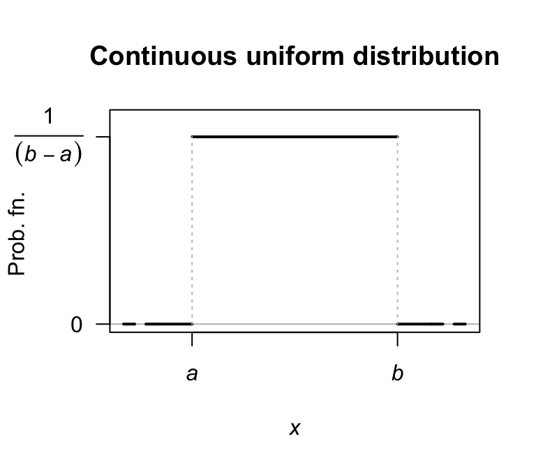
FIGURE 7.1: The PDF for a continuous uniform distribution \(U(a,b)\).
Definition 7.2 (Continuous uniform distribution: distribution function) For a random variable \(X\) with the continuous uniform distribution given in Eq. (7.1), the distribution function is \[ F_X(x; a, b) = \begin{cases} 0 & \text{for $x < a$};\\ \displaystyle \frac{x - a}{b - a} & \text{for $a \le x \le b$};\\ 1 & \text{for $x > b$}. \end{cases} \]
7.2.2 Properties
The following are the basic properties of the continuous uniform distribution.
Theorem 7.1 (Continuous uniform distribution properties) If \(X\sim\text{Unif}(a,b)\) then
- \(\operatorname{E}[X] = (a + b)/2\).
- \(\operatorname{var}[X] = (b - a)^2/12\).
- \(M_X(t) = \{ \exp(bt) - \exp(at) \} / \{t(b - a)\}\).
- The median is \((a + b)/2\).
Proof. These proofs are left as exercises.
The four R functions for working with the continuous uniform distribution have the form [dpqr]unif(., min, max) (see App. E):
-
dunif(x, min, max)computes the PDF at \(X = {}\)x; -
punif(q, min, max)computes the CDF at \(X = {}\)q; -
qunif(p, min, max)computes the quantile for cumulative probabilityp; and -
runif(n, min, max)generatesnrandom numbers,
where min\({} = a\) and max\({} = b\).
Example 7.1 (Continuous uniform) If \(X\) is uniformly distributed on \([-2, 2]\), then \(\Pr(|X| > \frac{1}{2})\) can be found (Fig. 7.2). Since \[ f_X(x; a = -2, b = 2) = \frac{1}{4} \quad\text{for $-2 < x < 2$}, \] then \[\begin{align*} \Pr\left(|X| > \frac{1}{2}\right) &= \Pr\left(X > (1/2)\right) + \Pr\left(X < -(1/2)\right)\\ &= \int^2_{1/2} f(x)\,dx + \int^{-1/2}_{-2} f(x)\,dx\\ &= 3/4. \end{align*}\] The probability could also be computed by finding the area of the appropriate rectangle. Alternatively, in R:
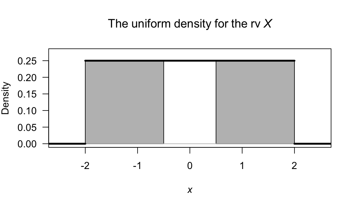
FIGURE 7.2: The random variable \(X\), with \(\Pr( |X| > 1/2)\) shaded.
7.3 Normal distribution
7.3.1 Definition
The most well-known continuous distribution is probably the normal distribution (or Gaussian distribution), sometimes called the bell-shaped distribution. The normal distribution has many applications (especially in sampling; see Sect. 12.4), and many natural quantities (such as heights and weights of humans) follow normal distributions.
Definition 7.3 (Normal distribution) If a random variable \(X\) has the PDF \[\begin{equation} f_X(x; \mu, \sigma^2) = \displaystyle \frac{1}{\sigma \sqrt{2\pi}} \exp\left\{ -\frac{1}{2}\left( \frac{x-\mu}{\sigma}\right)^2 \right\} \quad\text{for $-\infty<x<\infty$}, \tag{7.2} \end{equation}\] then \(X\) has a normal distribution. The two parameters are the mean \(\mu\) such that \(-\infty < \mu < \infty\); and the variance \(\sigma^2\) such that \(\sigma^2 > 0\). We write \(X\sim N(\mu, \sigma^2)\) or \(X\sim \text{Normal}(\mu, \sigma^2)\).
Some authors—especially in non-theoretical work—use the notation \(X\sim N(\mu,\sigma)\) (that is, the second argument is the standard deviation, rather than the variance) so it is wise to confirm the notation used.
Various normal distributions are shown in the visualisation below, for different values of \(\mu\) and \(\sigma\). For the same value of \(\mu\), larger values of \(\sigma\) show more variation in teh distribution (as expected).
FIGURE 7.3: Normal distributions.
In drawing the graph of the normal PDF, note that
- \(f_X(x)\) is symmetrical about \(\mu\): \(f_X(\mu - x) = f_X(\mu + x)\).
- \(f_X(x) \to 0\) asymptotically as \(x\to \pm \infty\).
- \(f_X'(x) = 0\) when \(x = \mu\), and a maximum occurs there.
- \(f_X''(x) = 0\) when \(x = \mu \pm \sigma\) (points of inflection).
The proof that \(\displaystyle \int^\infty_{-\infty} f_X(x)\,dx = 1\) is not obvious so will not be given. The proof relies on first squaring the integral and then changing to polar coordinates.
Definition 7.4 (Normal distribution: distribution function) For a random variable \(X\) with the normal distribution given in Eq. (7.2), the distribution function is \[\begin{align*} F_X(x; \mu, \sigma^2) &= \frac{1}{\sigma \sqrt{2\pi}} \int_{-\infty}^x \exp\left\{\frac{(t - \mu)^2}{2\sigma^2}\right\}\, dt\\ &= \frac{1}{2} \left\{1 + \operatorname{erf} \left( \frac{x - \mu}{\sigma {\sqrt{2}} }\right)\right\} \end{align*}\] where \(\operatorname{erf}(\cdot)\) is the error function \[\begin{equation} \operatorname{erf}(x) = \frac{2}{\sqrt{\pi}} \int _{0}^{x} \exp\left( -t^{2}\right)\,dt, \tag{7.3} \end{equation}\] for \(x \in\mathbb{R}\). The function \(\operatorname{erf}(\cdot)\) appears in numerous places, is commonly tabulated, and available in many computer packages.
7.3.2 Properties
The following are the basic properties of the normal distribution.
Theorem 7.2 (Normal distribution properties) If \(X\sim N(\mu,\sigma^2)\) then
- \(\operatorname{E}[X] = \mu\).
- \(\operatorname{var}[X] = \sigma^2\).
- \(M_X(t) = \displaystyle \exp\left(\mu t + \frac{t^2\sigma^2}{2}\right)\).
- The median is \(\mu\).
- The mode is \(\mu\).
Proof. The proof is delayed until after Theorem 7.3.
The four R functions for working with the normal distribution have the form [dpqr]norm(., mean, sd) (see App. E):
-
dnorm(x, mean, sd)computes the PDF at \(X = {}\)x; -
pnorm(q, mean, sd)computes the CDF at \(X = {}\)q; -
qnorm(p, mean, sd)computes the quantile for cumulative probabilityp; and -
rnorm(n, mean, sd)generatesnrandom numbers,
where mean\({} = \mu\) and sigma\({} = \sigma\).
Note that the normal distribution in R is specified by giving the standard deviation and not the variance.
The error function \(\operatorname{erf}(\cdot)\) is not available directly in R, but can be evaluated using
\[
\operatorname{erf}(x) = 2\times \texttt{pnorm}(x\sqrt{2}\,) - 1,
\]
since mean\({} = \mu = 0\) and sd\({} = \sigma = 1\) are the defaults.
7.3.3 The standard normal distribution
A special case of the normal distribution is the standard normal distribution, when the normal distribution has mean zero and variance one.
Definition 7.5 (Standardard normal distribution) The PDF for a random variable \(Z\) with a standard normal distribution, sometimes denoted \(\phi(x)\), is \[\begin{equation} f_Z(z) = \displaystyle \frac{1}{\sqrt{2\pi}} \exp\left\{ -\frac{z^2}{2}\right\} \tag{7.4} \end{equation}\] where \(-\infty < z < \infty\). We write \(Z\sim N(0, 1)\).
Since \(f_Z(z)\) is a PDF, then \[\begin{equation} \frac 1{\sqrt{2\pi}}\int^\infty_{-\infty} \exp\left\{-\frac{1}{2} z^2\right\}\,dz = 1, \tag{7.5} \end{equation}\] a result which proves useful in many contexts (as in the proof of the second statement in Theorem 6.7, and in the proof below).
Definition 7.6 (Standard normal distribution: distribution function) For a random variable \(X\) with the standard normal distribution given in Eq. (7.4), the distribution function is \[\begin{align} F_X(x) &= \frac{1}{2} \left\{1 + \operatorname{erf} \left( \frac {x}{\sqrt{2}} \right)\right\}\nonumber\\ &= \int_{-\infty}^z \frac{1}{\sqrt{2\pi}} \exp\left\{ -\frac{t^2}{2}\right\}\, dt\nonumber \\ &= \Phi(z) \tag{7.6} \end{align}\] where \(\operatorname{erf}(\cdot)\) is the error function (7.3).
The density and distribution functions for the standard normal distribution are used so often that they have their own notation. The density function is denoted \(\phi(\cdot)\), and the distribution function is denoted \(\Phi(\cdot)\). Then, the density function a normal distribution with mean \(\mu\) and standard deviation \(\sigma\) is \(\phi\big( (x - \mu)/\sigma\big)\), and the corresponding distribution function is \(\Phi\big( (x - \mu)/\sigma\big)\).
Note: \(\displaystyle\frac{d}{dx} \Phi(x) = \phi(x)\).
The following are the basic properties of the standard normal distribution.
Theorem 7.3 (Standard normal distribution properties) If \(Z\sim N(0, 1)\) then
- \(\operatorname{E}[Z] = 0\).
- \(\operatorname{var}[Z] = 1\).
- \(M_Z(t) = \displaystyle \exp\left(\frac{t^2}{2}\right)\).
Proof. Part 3 could be proven first, and used to prove Parts 1 and 2. However, proving Parts 1 and 2 directly is constructive. For the expected value: \[\begin{align*} \operatorname{E}[Z] &= \frac {1}{\sqrt{2\pi}} \int^\infty_{-\infty} z \exp\left\{-\frac{1}{2}z^2 \right\}\,dz\\ &= \int^\infty_{-\infty} -\frac{d}{dz} \left(\exp\left\{-\frac{1}{2}z^2\right\} \right)\, dz\\ &= \left[ -\exp\left\{-\frac{1}{2}z^2\right\}\right]^\infty_{-\infty} = 0, \end{align*}\] since the integrand is symmetric about \(0\).
For the variance, first see that \(\operatorname{var}[Z] = \operatorname{E}[Z^2] - \operatorname{E}[Z]^2 = \operatorname{E}[Z^2]\) since \(\operatorname{E}[Z] = 0\). So: \[ \operatorname{var}[X] = \operatorname{E}[Z^2] = \frac {1}{\sqrt{2\pi}}\int^\infty_{-\infty}z^2\, \exp\left(-\frac{1}{2}z^2\right)\,dz. \] To integrate by parts (i.e., \(\int u\,dv = uv - \int v\, du\)), set \(u = z\) (so that \(du = 1\)) and set \[ dv = z\exp\left(-\frac{1}{2}z^2\right) \quad\text{so that}\quad v = -\exp\left(-\frac{1}{2}z^2\right). \] Hence, \[\begin{align*} \operatorname{var}[X] &= \frac {1}{\sqrt{2\pi}} \left\{ -z \exp\left\{-\frac{1}{2}z^2\right\} - \int^\infty_{-\infty}-\exp\left\{-\frac{1}{2}z^2\right\}\, dz \right\}\\ &= \frac {1}{\sqrt{2\pi}}\left(\left. -z\,\exp\left\{-\frac{1}{2} z^2\right\}\right|^\infty_{-\infty}\right) + \frac{1}{\sqrt{2\pi}}\int^\infty_{-\infty} \exp\left\{-\frac{1}{2}z^2\right\}\,dz = 1 \end{align*}\] since the first term is zero, and the second term uses Eq. (7.5).
For the MGF: \[ M_Z(t) = \operatorname{E}[\exp\left\{tZ\right\}] = \int^\infty_{-\infty} \exp\left\{tz\right\} \frac{1}{\sqrt{2\pi}} \exp\left\{-\frac{1}{2}z^2\right\}\,dz. \] Collecting together the terms in the exponent and completing the square, \[\begin{equation*} -\frac{1}{2}[z^2 -2tz] = -\frac{1}{2}(z - t)^2+\frac{1}{2} t^2. \end{equation*}\] Taking the constants outside the integral: \[ M_Z(t) = \exp\left\{\frac{1}{2}t^2\right\}\int^\infty_{-\infty} \frac{1}{\sqrt{2\pi}} \exp\left\{-\frac{1}{2}[z - t]^2\right\}\,dz. \] The integral here is \(1\), since it is the area under an \(N(t, 1)\) PDF. Hence \[ M_Z(t) = \exp\left\{\frac{1}{2} t^2\right\}. \]
The standard normal distribution is important in practice since any normal distribution can be rescaled into a standard normal distribution using \[\begin{equation} Z = \frac{X - \mu}{\sigma}. \tag{7.7} \end{equation}\] Since \(Z = (X - \mu)/\sigma\), then \(X = \mu + \sigma Z\), and so \[ \operatorname{E}[X] = \operatorname{E}[\mu + \sigma Z] = \mu + \sigma \operatorname{E}[Z] = \mu \] because \(\operatorname{E}[Z] = 0\). Also \[ \operatorname{var}[X] = \operatorname{var}[\mu +\sigma Z] = \sigma^2\operatorname{var}[Z] = \sigma^2 \] because \(\operatorname{var}[Z] = 1\). Finally \[ M_X(t) = \operatorname{E}[\exp(tX)] = \operatorname{E}\big[\exp\{t(\mu + \sigma Z)\}\big] = \exp(\mu t)\operatorname{E}\big[\exp(t\sigma Z)\big]. \] However, \(\operatorname{E}\big[\exp(t\sigma Z)\big] = M_Z(t\sigma) = \exp\left\{\frac{1}{2}(\sigma t)^2\right\}\) so \[ M_Z(t) = \displaystyle \exp\left(\frac{t^2}{2}\right). \]
7.3.4 Determining normal probabilities
The probability \(\Pr(a < X \le b)\) where \(X\sim N(\mu, \sigma^2)\) can be written
\[
\Pr(a < X \le b) = F_X(b) - F_X(a).
\]
where \(F_X(x)\) is the distribution function in Def. 7.6.
The integral in the distribution function cannot be written in terms of standard functions and in general must be evaluated for a particular \(x\) numerically (e.g., using Simpson’s rule or similar).
However, all statistical packages have built-in procedures to evaluate \(F_X(x)\) for any \(z\) (such as pnorm() in R).
Also, since any normal distribution can be transformed into a standard normal distribution, we can write \[ z_1 = (a - \mu)/\sigma \quad\text{and}\quad z_2 = (b - \mu)/\sigma \] and hence the probability is \[ \Pr( z_1 < Z \le z_2) = \Phi(z_2) - \Phi(z_1), \] where \(\Phi(z)\) is the distribution function for the standard normal distribution, as in Eq. (7.3).
The process of converting a value \(x\) into \(z\) using \(z = (x - \mu)/\sigma\) is called standardising. Tables of \(\Phi(z)\) (or sometimes \(1 - \Phi(z)\)) are commonly available. These tables can be used to compute any probabilities associated with the normal distributions (see the examples below). Of course, R can be used too.
In addition, the tables are often used in the reverse sense, where the probability of an event is given and the value of the random variable is sought.
In these case, the tables are used ‘backwards’; the appropriate area is found in the body of the table and the corresponding \(z\)-value found in the table margins.
In R, the function qnorm() is used.
This \(z\)-value is then converted to a value of the original random variable using
\[\begin{equation}
x = \mu + z\sigma.
\tag{7.8}
\end{equation}\]
This process is sometimes referred to as unstandardising.
The following examples illustrate the use of R. Drawing rough graphs showing the relevant areas is encouraged.
Example 7.2 (Walking speeds) A study of stadium evacuations used a simulation to compare scenarios (Xie et al. 2017). The walking speed of people was modelled using a \(N(1.15, 0.2^2)\) distribution; that is, \(\mu = 1.15\) m/s with a standard deviation of \(0.2\) m/s. The situation can be shown in Fig. 7.4, top left panel.
Many questions can be asked about the walking speeds, and R used to compute answers. Using this model:
- What is the probability that a person walks faster than \(1.5\) m/s?
- What is the probability that a person walks slower than \(1.0\) m/s?
- What is the probability that a person walks between \(1.0\) m/s and \(1.5\) m/s?
- At what speed do the slowest \(15\)% of people walk?
- At what speed do the quickest \(5\)% of people walk?
Sketches of each of these situations are shown in Fig. 7.4. Using R:
# Part 1
1 - pnorm(1.5, mean = 1.15, sd = 0.2)
#> [1] 0.04005916

# Part 2
pnorm(1, mean = 1.15, sd = 0.2)
#> [1] 0.2266274

# Part 3
pnorm(1.5, mean = 1.15, sd = 0.2) -
   pnorm(1, mean = 1.15, sd = 0.2)
#> [1] 0.7333135

# Part 4
qnorm(0.15, mean= 1.15, sd = 0.2)
#> [1] 0.9427133

# Part 5
qnorm(0.95, mean = 1.15, sd = 0.2)
#> [1] 1.478971
So the answers are, respectively:
- 4%;
- 22.7%;
- 73.3%;
- 0.894 m/s;
- 1.479m/s.
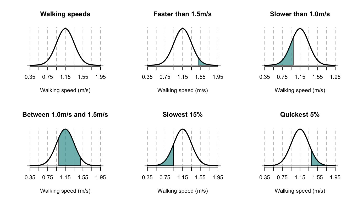
FIGURE 7.4: The normal distribution used for modelling walking speeds. The vertical dotted lines are at the mean and \(\pm1\), \(\pm2\), \(\pm3\) and \(\pm4\) standard deviations from the mean.
Example 7.3 (Using normal distributions) Scores on an examination have a normal distribution, with a mean score of \(50\) and standard deviation of \(10\). Suppose the top \(75\)% of candidates taking this examination are to be passed; call the minimum passing score \(x^*\).
Since \(X\sim N(50, 10^2)\): \[\begin{align*} \Pr(X > x^*) &= 0.75\\ \Pr\left(Z > \frac{x^* - 50}{10}\right) &= 0.75\\ \Pr\left(Z < \frac{50 - x^*}{10}\right) & = 0.75. \end{align*}\] From tables, \(0.75 = \Phi(0.675)\) so \((50 - x^*)/10 = 0.675\) and \(x^* = 43.25\). Using R:
qnorm(0.25, # 'Top 75%' is the same as the 'bottom 25%'
      mean = 50,
      sd = 10)
#> [1] 43.2551
7.3.5 Normal approximation to the binomial
In Sect. 6.4, the binomial distribution was considered. Sometimes using the binomial distribution is tedious; consider a binomial random variable \(X\) where \(n = 1000\), \(p = 0.45\) and \(\Pr(X > 650)\) is sought: we would calculate \(\Pr(X = 651) + \Pr(X = 652) + \cdots + \Pr(X = 1000)\).
However, sometimes the normal distribution can be used to approximate binomial probabilities. For certain parameter values, the binomial pf starts to take on a normal distribution shape (Fig. 7.5).
When is the binomial probability function close enough to use the normal approximation? There is no definitive answer; a common guideline suggests that if both \(np \ge 5\) and \(n(1 - p) \ge 5\) the approximation is satisfactory. (These are only guidelines, and other texts may suggest different guidelines.)
Figure 7.5 shows some picture of various binomial probability functions overlaid with the corresponding normal distribution; the approximation is visibly better as the guidelines given above are satisfied.
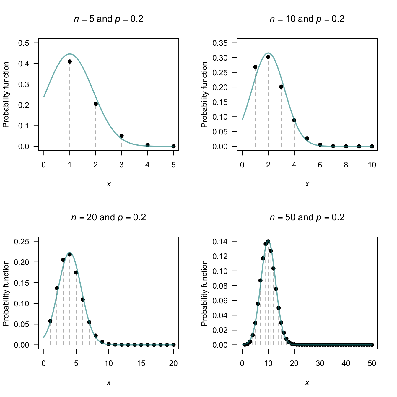
FIGURE 7.5: The normal distribution approximating a binomial distribution. The guidelines suggest the approximation should be good when \(np \ge 5\) and \(n (1 - p) \ge 5\); this is evident from the pictures. In the top row, a significant amount of the approximating normal distribution even appears when \(Y < 0\).
The normal distribution can be used to approximate probabilities in situations that are actually binomial. A fundamental difficulty with this approach is that a discrete distribution is being modelled with a continuous distribution. This is best explained through an example. The example explains the principle; the idea extends to all situations where the normal distribution is used to approximate a binomial distribution.
If the random variable \(X\) has the binomial distribution \(X \sim \text{Bin}(n, p)\), the probability function can be approximated by the normal distribution \(Y \sim N(\mu, \sigma^2)\), where \(\mu = np\) and \(\sigma^2 = np(1 - p)\).
The approximation is good if both \(np \ge 5\) and \(n(1 - p) \ge 5\).
Example 7.4 (Normal approximation to binomial) Consider mdx mice (which have a strain of muscular dystrophy) from a particular source for which \(30\)% of the mice survive for at least \(40\) weeks. One particular experiment requires at least \(35\) of the \(100\) mice to live beyond \(40\) weeks. What is the probability that \(35\) or more of the group will survive beyond \(40\) weeks?
First see that the situation is binomial; if \(X\) is the number of mice from the group of \(100\) that survive, then \(X \sim \text{Bin}(100, 0.3)\). This could be approximated by the normal distribution \(Y\sim N(30, 21)\), where the variance is \(np(1 - p) = 100\times 0.3\times 0.7 = 21\). Both \(np = 30\) and \(n(1 - p) = 70\) are much larger than \(5\), so this approximation is expected to adequate.
Figure 7.6 shows the upper tail of the distribution near \(X = 35\): using the normal approximation from \(Y = 35\), only half of the original bar in the binomial pf is included. However, since the number of mice is discrete, we want the entire bar corresponding to \(X = 35\). So to compute the correct answer, the normal distribution must be evaluated for \(\Pr(Y > 34.5)\). This change from \(Y \ge 34.5\) to \(Y > 34.5\) is called using the continuity correction.
The exact answer (using the binomial distribution) is \(0.1629\) (rounded to four decimal places). Using the normal distribution with the continuity correction gives the answer as \(0.1631\); using the normal distribution without the continuity correction, the answer is \(0.1376\). The solution is more accurate, as expected, using the continuity correction.
# Exact
ExactP <- sum( dbinom(x = 35:100,
                      size = 100,
                      prob = 0.30))
ExactP2 <- 1 - pbinom(34,
                      size = 100,
                      prob = 0.30)
# Normal approx
NormalP <- 1 - pnorm(35,
                     mean = 30,
                     sd = sqrt(21))
# Normal approx with continuity correction
ContCorrP <- 1 - pnorm(34.5,
                       mean = 30,
                       sd = sqrt(21))
cat("Exact:" = round(ExactP, 6), "\n") # \n means "new line"
#> 0.162858
cat("Exact (alt):" = round(ExactP2, 6), "\n")
#> 0.162858
cat("Normal approx:" = round(NormalP, 6), "\n")
#> 0.137617
cat("With correction:" = round(ContCorrP, 6), "\n")
#> 0.163055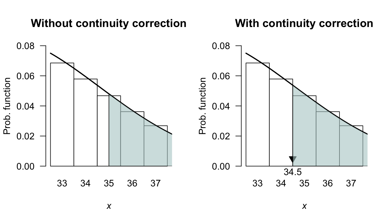
FIGURE 7.6: The normal distribution approximating the binomial distribution when \(n = 100\), \(p = 0.3\) and finding the probability that \(X > 35\).
Example 7.5 (Continuity correction) Consider rolling a standard die \(100\) times, and counting the number of times a ![]() appear uppermost.
The random variable \(X\) is the number of times a
appear uppermost.
The random variable \(X\) is the number of times a ![]() appears; then, \(X\sim \text{Bin}(n = 100, p = 1/6)\).
appears; then, \(X\sim \text{Bin}(n = 100, p = 1/6)\).
Since \(np = 16.667\) and \(n(1 - p) = 83.333\) are both greater than \(5\), a normal approximation should be accurate, so define \(Y\sim N(16.6667, 13.889)\) (where the variance is \(np(1 - p) = 13.889\)). Various probabilities (Table 7.1) show the accuracy of the approximation, and the way in which the continuity correction has been used.
You should understand how the concept of the continuity correction has been applied in each situation, and be able to compute the probabilities for the normal approximation.
| Event (binomial) | Prob (binomial) | Event (normal) | Prob (normal) | |
|---|---|---|---|---|
| \(\Pr(X \lt 10)\) | 0.0213 | \(\Pr(Y \lt 9.5)\) | 0.0368 | |
| \(\Pr(X \le 15)\) | 0.3877 | \(\Pr(Y \lt 15.5)\) | 0.3771 | |
| \(\Pr(X \gt 17)\) | 0.4006 | \(\Pr(Y \gt 17.5)\) | 0.4115 | |
| \(\Pr(X \ge 21)\) | 0.1519 | \(\Pr(Y \gt 20.5)\) | 0.1518 | |
| \(\Pr(15 \lt X \le 17)\) | 0.2117 | \(\Pr(15.5 \lt Y \lt 17.5)\) | 0.2113 | |
| \(\Pr(15 \le X \le 17)\) | 0.3120 | \(\Pr(14.5 \lt Y \lt 17.5)\) | 0.2017 |
7.4 Exponential distribution
The normal distribution is defined for all real values, but many quantities are defined on the positive real numbers only. This is not always a problem, especially when the observations are far from zero, such as heights of adult humans. However, many random variables have observations close to zero, and the data are often skewed to the right (positively skewed).
Many distributions can be used for modelling right-skewed data defined on the positive real numbers; the simplest is the exponential distribution.
7.4.1 Derivation and definition
The exponential distribution is closely related to the Poisson distribution. To show this, consider a Poisson process (Sect. 6.7.1), where events occur at an average rate of \(\lambda\) events per unit time (e.g., \(\lambda = 0.5\) per minute).
Then consider a fixed length of time \(t > 0\); then, the number of occurrences \(Y\) would have an average rate of \(\lambda t\) (e.g., in 12 minutes, we’d expect an average rate of \(0.5\times 12 = 6\) occurrences). That is, the number of events occurring in the interval \((0, t)\) has Poisson distribution with mean \(\lambda t\), with probability function \[\begin{equation} p_Y(y) = \frac{\exp(-\lambda t) (\lambda t)^y}{y!} \quad \text{for $y = 0, 1, 2, \dots$}. \tag{7.9} \end{equation}\] Hence, the probability that zero events occur in the interval \((0, t)\) is \[ \Pr(Y = 0) = \frac{\exp(-\lambda t) (\lambda t)^0}{0!} = \exp(-\lambda t) \] using \(Y = 0\) in Eq. (7.9).
Now, introduce a new random variable \(T\) that represent the time until the first event occurs. Then, \(Y = 0\) (i.e., no events occur in the interval \((0, t)\)) corresponds to \(T > t\) (i.e., the time till the first event occurs must be great than the time interval \(t\)). That is, \[ \Pr(Y = 0) = \exp(-\lambda t) = \Pr(T > t). \] Rewriting in terms of a distribution function for \(T\), \[ F_T(t) = 1 - \Pr(T > t) = 1 - \exp(-\lambda t) \] for \(t > 0\). Hence, the probability density function is \[ f_T(t) = \lambda \exp(-\lambda t) \] for \(t > 0\). This is the probability density function for the exponential distribution.
This shows that if events occur at random according to a Poisson distribution, then the time (or the space) between those events follows an exponential distribution (Theorem 7.4). Hence the exponential distribution is used to describe the interval between consecutive randomly occurring events that follow a Poisson distribution.
Theorem 7.4 (Poisson process and exponential distributions) Consider a Poisson process at rate \(\lambda\) and suppose observation starts at an arbitrary time point. Then the time \(T\) to the first event has an exponential distribution with mean \(\operatorname{E}[T] = 1/\lambda\); i.e., \[ f_T(t) = \lambda \exp(-\lambda t),\quad t > 0. \]
Although the theorem refers to ‘time’, the variable of interest may be distance or any other continuous variable measuring the interval between events.
If events occur according to a Poisson distribution with rate \(\lambda\), then the time between the Poisson events can be modelled using an exponential distribution with rate \(\lambda\).
For example, if events occur with a Poisson distribution at a rate of \(\lambda = 5\) events per day, then the time between events can be modelled with an exponential distribution with \(\lambda = 5\).
The exponential distribution is usually written as follows.
Definition 7.7 (Exponential distribution) If a random variable \(X\) has the PDF \[\begin{equation} f_X(x; \lambda) = \lambda \exp(-\lambda x) \quad \text{for $x > 0$}. \tag{7.10} \end{equation}\] then \(X\) has an exponential distribution with rate parameter \(\lambda > 0\). We write \(X\sim\text{Exp}(\lambda)\) or \(X\sim\text{Exp}(\text{rate} = \lambda)\). This is called the rate parameterisation.
Equivalently, we can define \(\beta = 1/\lambda\) as the scale parameter and write \[\begin{equation} f_X(x; \beta) = \frac{1}{\beta} \exp(-x/\beta) \quad \text{for $x > 0$} \tag{7.11} \end{equation}\] then \(X\) has an exponential distribution with scale parameter \(\beta > 0\). We write \(X\sim\text{Exp}(\beta)\) or \(X\sim\text{Exp}(\text{scale} = \beta)\). This is called the scale parameterisation.
Various exponential distributions are shown in the visualisation below, for different values of \(\lambda = 1/\beta\).
FIGURE 7.7: Exponential distributions.
Definition 7.8 (Exponential distribution: distribution function) For a random variable \(X\) with the exponential distribution given in Def. 7.7, the distribution function is \[\begin{align*} F_X(x; \lambda) &= 1 - \exp\left\{-\lambda x\right\} \quad\text{(rate parameterisation)}\\ F_X(x; \beta) &= 1 - \exp\left\{-x/\beta\right\} \quad\text{(scale parameterisation)} \end{align*}\] for \(x > 0\).
7.4.2 Properties
The following are the basic properties of the exponential distribution.
Theorem 7.5 (Exponential distribution properties) If \(X\sim\text{Exp}(\beta)\) then
- \(\operatorname{E}[X] = \beta = 1/\lambda\).
- \(\operatorname{var}[X] = \beta^2 = 1/\lambda^2\).
- \(M_X(t) = (1 - \beta t)^{-1}\) for \(t < 1/\beta\) (or, \(M_X(t) = \lambda/(\lambda - t)\) for \(t < \lambda\)).
- The median is \(\beta\log 2\).
Proof. The proofs are left as an exercise.
The parameter \(\beta\) represents the mean of the exponential distribution. The alternative parameter \(\lambda = 1/\beta\) represents the mean rate at which events occur. Like the Poisson distribution, the variance is defined once the mean is defined .
The four R functions for working with the exponential distribution have the form [dpqr]exp(., rate) (see App. E):
-
dexp(x, rate)computes the PDF at \(X = {}\)x; -
pexp(q, rate)computes the CDF at \(X = {}\)q; -
qexp(p, rate)computes the quantile for cumulative probabilityp; and -
rexp(n, rate)generatesnrandom numbers,
where rate\({} = \lambda = 1/\beta\).
Example 7.6 (Exponential distributions) Allen et al. (1975) use the exponential distribution to model daily rainfall in Kentucky.
Example 7.7 (Exponential distributions) Cox and Lewis (1966) give data collected by Fatt and Katz concerning the time intervals between successive nerve pulses along a nerve fibre. There are \(799\) observations which we do not give here. The mean time between pulses is \(\beta = 0.2186\) seconds. An exponential distribution might be expected to model the data well. This is indeed the case (Fig. 7.8).
Define \(X\) as the time between successive nerve pulses (in seconds); then \(X\sim \text{Exp}(\beta = 0.2186)\) (so the rate parameter is \(\lambda = 1/0.2186 = 4.575\) per second). To find the proportion of time intervals longer than \(1\) second: \[\begin{align*} \Pr(X > 1) &= \int_1^\infty \frac{1}{0.2186}\exp(-x/0.2186)\, dx \\ &= \left[-\exp(-x/0.2186)\right]_1^\infty \\ &= 0.01031. \end{align*}\] There is about a \(1\)% chance of a nerve pulse exceeding one second.
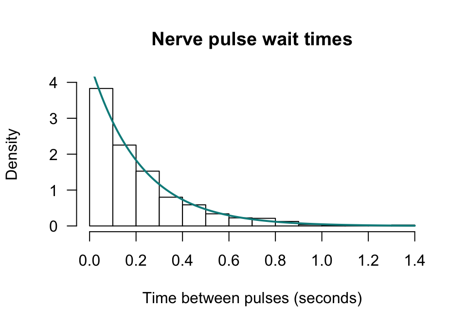
FIGURE 7.8: The time between successive nerve pulses. An exponential distribution fits well.
The relationship between the Poisson and exponential distribution was explored in Sect. 7.4.1 (see, for example, Theorem 7.4). The next example explores this relationship
Example 7.8 (Relationship between exponential and Poisson distributions) Suppose a Poisson process occurs at the mean rate of \(5\) events per hour. Let \(N\) represent the number of events in one day and \(T\) the time between consecutive events. We can describe the distribution of the time between consecutive events and the distribution of the number of events in one day (\(24\,\text{h}\)).
Since events occur at the mean rate of \(\lambda = 5\) events per hour, the mean time between consecutive events is \(\beta = 1/\lambda = 0.2\,\text{h}\). Hence, the mean number of events in one day is \(\mu = 24\times 5 = 120\).
Consequently, \(N\sim\text{Poisson}(\mu = 120)\) and \(X\sim\text{Exp}(\beta = 0.2)\) (or, equivalently, \(X\sim\text{Exp}(\lambda = 5)\)).
An important feature of a Poisson process, and hence of the exponential distribution, is the memoryless or Markov property: the future of the process at any time point does not depend on the history of the process. This property is captured in the following theorem.
Theorem 7.6 (Memoryless property) If \(T \sim \text{Exp}(\lambda)\) where \(\lambda\) is the rate parameter, then for \(s > 0\) and \(t > 0\), \[ \Pr(T > s + t \mid T > s) = \Pr(T > t) \]
Proof. Using Definition 3.17, \[ \Pr(T > s + t \mid T > s) = \frac{ \Pr( \{T > s + t\} \cap \{T > s\})} {\Pr(T > s)} \] But if \(T > s + t\), then \(T > s\). Consequently \(\Pr( \{T > s + t \}\cap \{T > s \} ) = \Pr(T > s + t)\) and so \[\begin{align*} \Pr(T > s + t \mid T > s ) &= \frac{\Pr(T > s +t )}{\Pr(T > s)}\\ &= \frac{\exp\left\{-\lambda(s + t)\right\}}{\exp\left\{-\lambda s\right\}}\\ &= \exp\left\{-\lambda t\right\}\\ &= \Pr(T > t). \end{align*}\]
This theorem states that the probability that the time to the next event is greater than \(t\) does not depend on the time \(s\) back to the previous event. This is called the memoryless property of the exponential distribution.
Example 7.9 (Memoryless property of exponential distribution) Suppose the lifespan of component \(A\) is modelled by an exponential distribution with mean \(12\) months. Then, \(T \sim \text{Exp}(\beta = 6)\).
The probability that component \(A\) fails in less than \(6\) months is \[ \Pr(T < 6) = 1 - \exp(-6/12) = 0.3935. \]
Now, suppose component \(A\) has been in place for \(12\) months. The probability that it will fail in less than a further \(6\) months is \[ \Pr(T < 18 \mid T > 12) = \Pr(T < 6) = 1 - \exp(-6/12) = 0.3935 \] by the memoryless property.
Example 7.9 shows that an exponential process is ‘ageless’: the risk of ‘mortality’ remains constant with age. That is, the probability of such an event occurring in the next small interval, whether the failure of a component or the occurrence of an accident, remains constant regardless of the age of the component or the length of time since the last accident. In this sense, an exponential lifetime is different from a human lifetime, or the lifetime of many man-made objects, where the risk of ‘death’ in the next small interval increases with age.
7.5 Gamma distribution
7.5.1 Definition
Once the mean of an exponential distribution is defined, the variance is defined. More flexibility is sometimes needed, which is provided by the gamma distribution.
Definition 7.9 (Gamma distribution) If a random variable \(X\) has the PDF \[ f_X(x; \alpha, \beta) = \frac{x^{\alpha - 1}}{\beta^\alpha\, \Gamma(\alpha)} \exp(-x/\beta) \quad \text{for $x > 0$} \] then \(X\) has a gamma distribution, where \(\Gamma(\cdot)\) is the gamma function (see Sect. 6.11) and \(\alpha, \beta > 0\). The parameter \(\alpha\) is called the shape parameter and \(\beta\) is called the scale parameter. We write \(X \sim \text{Gamma}(\alpha, \beta)\) or \(X \sim \text{Gamma}(\text{shape} = \alpha, \text{scale} = \beta)\). This is called the scale parameterisation or the shape–scale parameterisation.
Equivalently, we can define \(\lambda = 1/\beta\) as the rate parameter and write \[ f_X(x; \alpha, \lambda) = \frac{\lambda^{\alpha}}{\Gamma(\alpha)} x^{\alpha - 1} \exp(-\lambda x) \quad \text{for $x > 0$}. \] We write \(X \sim \text{Gamma}(\alpha, \lambda)\) or \(X \sim \text{Gamma}(\text{shape} = \alpha, \text{rate} = \lambda)\). This is called the rate parameterisation or the shape–rate parameterisation.
The exponential distribution is a special case of the gamma distribution when the shape parameter is \(\alpha = 1\). This means that properties of the exponential distribution can be obtained by substituting \(\alpha = 1\) into the equivalent expression for the gamma distribution. That is, \[ \text{Exp}(\beta) = \text{Gamma}(1, \text{scale} = \beta) \quad \text{and} \quad \text{Exp}(\lambda) = \text{Gamma}(1, \text{rate} = \lambda). \]
In broad terms, the shape parameter dictates the general shape of the distribution; the scale parameter dictates how ‘stretched out’ the distribution is. Some texts use different notation for the shape and scale parameters. Some text also use a rate parameter \(1/\beta\) instead of a scale parameter. Sometimes we write \(X \sim \text{Gamma}(\text{shape} = \alpha, \text{scale} = \beta)\) when clarification of the parameterisation is necessary.
In R, the gamma function \(\Gamma(x)\) is evaluated using gamma(x).
The four R functions for working with the gamma distribution can be specified using either the rate or the scale parameterisation (see App. E).
The functions for the rate paramaterisation have the form [dpqr]gamma(., shape, rate):
-
dgamma(x, shape, rate)computes the PDF at \(X = {}\)x; -
pgamma(q, shape, rate)computes the CDF at \(X = {}\)q; -
qgamma(p, shape, rate)computes the quantile for cumulative probabilityp; and -
rgamma(n, shape, rate)generatesnrandom numbers,
where shape\({}= \alpha\) and rate\({}= \lambda = 1/\beta\).
The functions for the scale paramaterisation are
-
dgamma(x, shape, scale)computes the PDF at \(X = {}\)x; -
pgamma(q, shape, scale)computes the CDF function at \(X = {}\)q; -
qgamma(p, shape, scale)computes the quantile for cumulative probabilityp; and -
rgamma(n, shape, scale)generatesnrandom numbers,
where shape\({}= \alpha\) and scale\({}= \beta = 1/\lambda\) (see App. E).
The R functions are used in the same way, but explicitly specifying the scale input rather than the rate input; for example:
-
dgamma(x, shape, scale)computes the probability function at \(X = {}\)x.
Various gamma distributions are shown in the visualisation below, for different values of \(\alpha\) and \(\beta\).
FIGURE 7.9: Gamma distributions.
Notice that \[\begin{align} \int_0^\infty f_X(x)\,dx &= \int_0^\infty\frac{\exp(-x/\beta)\,x^{\alpha - 1}}{\beta^\alpha\Gamma(\alpha)}\,dx\nonumber\\ &= \frac{1}{\Gamma(\alpha)} \int_0^\infty \exp(-y)\, y^{\alpha-1}\,dy \quad \text{(on putting $y = x/\beta$)}\nonumber \\ &= 1, \tag{7.12} \end{align}\] because \(\int_0^\infty \exp(-y) y^{\alpha-1}\,dy = \Gamma(\alpha)\) is the gamma function.
7.5.2 Properties
The distribution function for the gamma distribution is complicated, involving incomplete gamma functions, and will not be given. The following are the basic properties of the gamma distribution.
Theorem 7.7 (Gamma distribution properties) If \(X\sim\text{Gamma}(\alpha, \beta)\) then
- \(\operatorname{E}[X] = \alpha\beta = \alpha/\lambda\).
- \(\operatorname{var}[X] = \alpha\beta^2 = \alpha/\lambda^2\).
- \(M_X(t) = (1 - \beta t)^{-\alpha}\) for \(t < 1/\beta\) (scale parameterisation), or \(M_X(t) = (1 - t/\lambda)^{-\alpha}\) for \(t < \lambda\) (rate parameterisation).
Proof. For the expected value: \[ \operatorname{E}[X] = \int_0^{\infty}x\, f_X(x)\,dx = \beta \frac{\Gamma(\alpha + 1)}{\Gamma(\alpha)} \underbrace{\int_0^{\infty}\frac{\exp(-x/\beta) x^{(\alpha + 1) - 1}}{\beta^{\alpha + 1}\Gamma(\alpha + 1)} \, dx}_{= 1} = \alpha\beta. \] This result follows from using Eq. (7.12) and Theorem 7.7 \[ \operatorname{E}[X^2] = \int_0^{\infty}x^2\, f_X(x) \, dx = \beta^2\frac{\Gamma(\alpha + 2)}{\Gamma(\alpha)} \underbrace{\int_0^{\infty}\frac{\exp(-x/\beta) x^{(\alpha + 2) - 1}}{\beta^{\alpha + 2}\Gamma(\alpha + 2)}\,dx}_{= 1} = \alpha(\alpha + 1)\beta^2 \] where the result follows by writing \(\Gamma(\alpha + 2) = (\alpha + 1)\alpha\Gamma(\alpha)\). Hence \[ \operatorname{var}[X] = \operatorname{E}[X^2] - (\operatorname{E}[X])^2 = \alpha(\alpha + 1)\beta^2 - (\alpha\beta)^2 = \alpha\beta^2 \] Also: \[\begin{align*} M_X(t) = \operatorname{E}[\exp(Xt)] &= \int_0^{\infty}\exp(tx) \frac{\exp(-x/\beta) x^{\alpha - 1}}{\beta^{\alpha} \Gamma(\alpha)} \, dx\\ &= \int_0^{\infty} \frac{\exp\{-x(1 - \beta t)/\beta\}x^{\alpha - 1}}{\beta^{\alpha}\Gamma(\alpha)} \, dx\\ &= \int_0^{\infty} \frac{\exp(-z) z^{\alpha - 1}}{\Gamma(\alpha)(1 - \beta t)^{\alpha - 1}} \, \frac{dz} {1 - \beta t}, \text{putting $z = x(1 - \beta t)/\beta$}\\ &= (1 - \beta t)^{-\alpha}, \end{align*}\] since the integral remaining is \(1\).
As usual the moments can be found by expanding \(M_X(t)\) as a series. That is, \[ M_X(t) = 1 + \alpha\beta t + \frac{\alpha(\alpha+1)\beta^2}{2!} t^2 + \cdots \] from which \[\begin{align*} \operatorname{E}[X] &= \text{coefficient of }t =\alpha\beta,\\ \operatorname{E}[X^2] &= \text{coefficient of }t^2/2!=\alpha(\alpha+1)\beta^2, \end{align*}\] as found earlier.
As for the normal distribution, the distribution function of the gamma cannot, in general, be computed without using numerical integration, tables (although see Example 7.11) or software.
A useful property of the gamma distribution is that the sum of \(n\) independent \(\text{Gamma}(\alpha_i, \beta)\) distributions has the gamma distribution \(\text{Gamma}\left(\sum_{i=1}^n \alpha_i, \beta\right)\). This is shown in Exercise 9.3.
Example 7.10 (Rainfall) Das (1955) used a (truncated) gamma distribution for modelling daily precipitation in Sydney. A similar approach is adopted by Wilks (1990).
Larsen and Marx (1986) (Case Study 4.6.1) use the gamma distribution to model daily rainfall in Sydney, Australia using the parameter estimates \(\alpha = 0.105\) and \(\beta = 76.9\) (based on Das (1955)). The comparison between the data and the model (Table 7.2) indicates a good agreement between the data and the theoretical distribution.
| Rainfall (mm) | Observed | Modelled | Rainfall (mm) | Observed | Modelled | |
|---|---|---|---|---|---|---|
| 0–5 | 1631 | 1639 | 46–50 | 18 | 12 | |
| 6–10 | 115 | 106 | 51–60 | 18 | 20 | |
| 11–15 | 67 | 62 | 61–70 | 13 | 15 | |
| 16–20 | 42 | 44 | 71–80 | 13 | 12 | |
| 21–25 | 27 | 32 | 81–90 | 8 | 9 | |
| 26–30 | 26 | 26 | 91–100 | 8 | 7 | |
| 31–35 | 19 | 21 | 101–125 | 16 | 12 | |
| 36–40 | 14 | 17 | 126–150 | 7 | 7 | |
| 41–45 | 12 | 14 | 151–425 | 14 | 13 |
Example 7.11 (Electrical components) The lifetime of an electrical component in hours, say \(T\), can be well modelled by the distribution \(\text{Gamma}(2, 1)\). What is the probability that a component will last for more than three hours?
From the information, \(T\sim \text{Gamma}(\alpha = 2, \beta = 1)\). The required probability is therefore \[\begin{align*} \Pr(T > 3) &= \int_3^\infty \frac{1}{1^2 \Gamma(2)}t^{2 - 1} \exp(-t/1)\,dt \\ &= \int_3^\infty t \exp(-t)\,dt \end{align*}\] since \(\Gamma(2) = 1! = 1\). This expression can be integrated using integration by parts: \[\begin{align*} \Pr(T > 3) &= \int_3^\infty t \exp(-t)\,dt \\ &= \left[ -t \exp(-t)\right]_3^\infty - \int_3^\infty -\exp(-t)\, dt \\ &= [ (0) - \{-3\exp(-3)\}] - \left[ \exp(-t)\right]_3^\infty \\ &= 3\exp(-3) + \exp(-3)\\ &= 0.1991 \end{align*}\] Integration by parts is only possible since \(\alpha\) is an integer. If \(\alpha = 2.5\), for example, integration by parts would not be possible.
A more general approach is to use tables of the incomplete gamma function to evaluate the integral, numerical integration, or software. To use R:
# Integrate
integrate(dgamma, # The gamma distribution prob. fn
          lower = 3,
          upper = Inf,  # "Inf" means "infinity"
          shape = 2,
          scale = 1)
#> 0.1991483 with absolute error < 9.3e-05

# Directly
1 - pgamma(3,
           shape = 2,
           scale = 1)
#> [1] 0.1991483
Using any method, the probability is about \(20\)%.
Example 7.12 (MGFs for gamma and exponential distributions) If \(X_i\sim \text{Exponential}(\lambda)\) where \(\lambda\) is the rate, find the distribution of \(Y = X_1 + X_2 + \cdots + X_n\).
Since \(X\) has an exponential distribution, \(M_X(t) = (1 - t/\lambda)^{-1}\). Now, \[\begin{align*} M_Y(t) &= \operatorname{E}[\exp(tY)] \qquad\text{by definition of the MGF}\\ &= \operatorname{E}[\exp(t (X_1 + X_2 + \cdots + X_n))] \\ &= \operatorname{E}[\exp(t X_1) \cdot \exp(t X_2) \cdots \exp(t X_n)] \quad\text{(since $\exp(a + b) = \exp(a) \cdot \exp(b)$})\\ &= \operatorname{E}[\exp(t X_1)] \cdots \operatorname{E}[\exp(t X_n)] \quad\text{(by independence)}\\ &= [M_X(t)]^n \quad\text{(since all $X_i$ are identically distributed)}\\ &= (1 - t/\lambda)^{-n}. \end{align*}\] This is just the MGF for the gamma random variable \(\text{Gamma}(n, \lambda)\) (written using the rate parameterisation). Since MGFs uniquely determine distributions, \(Y \sim \text{Gamma}(n, \lambda)\).
7.6 Log-normal distribution
7.6.1 Definition
The log-normal distribution arises naturally as the distribution of a positive random variable \(X\) whose logarithm \(Y = \log X\) follows a normal distribution. Because \(X\) is strictly positive and right-skewed, the log-normal distribution is a natural model for quantities such as incomes, rainfall amounts, and survival times
Definition 7.10 (Log-normal distribution) A random variable \(X\) has a log-normal distribution if \(Y = \log X\) has a normal distribution. That is, \(X \sim \text{LogNormal}(\mu, \sigma^2)\) if and only if \(\log X \sim N(\mu, \sigma^2)\).
The PDF of \(X\) is \[ f_X(x;\, \mu, \sigma^2) = \frac{1}{x\,\sigma\sqrt{2\pi}} \exp\!\left\{-\frac{(\log x - \mu)^2}{2\sigma^2}\right\}, \quad \text{for $x > 0$}, \] where \(\mu \in \mathbb{R}\) is the log-mean (the mean of \(\log X\)) and \(\sigma^2 > 0\) is the log-variance (the variance of \(\log X\)). We write \(X \sim \text{LogNormal}(\mu, \sigma^2)\).
If \(X \sim \text{LogNormal}(\mu, \sigma^2)\) then \(\log X \sim N(\mu, \sigma^2)\). Conversely, if \(Z \sim N(\mu, \sigma^2)\) then \(\exp Z \sim \text{LogNormal}(\mu, \sigma^2)\). The parameters \(\mu\) and \(\sigma^2\) are the mean and variance of the logarithm of \(X\), not of \(X\) itself.
In R, the four functions for working with the log-normal distribution have the form [dpqr]lnorm(., meanlog, sdlog) (see App. E):
-
dlnorm(x, meanlog, sdlog)computes the PDF at \(X = {}\)x; -
plnorm(q, meanlog, sdlog)computes the CDF at \(X = {}\)q; -
qlnorm(p, meanlog, sdlog)computes the quantile for cumulative probabilityp; and -
rlnorm(n, meanlog, sdlog)generatesnrandom numbers,
where meanlog \({}= \mu\) and sdlog \({}= \sigma\) (note: the standard deviation, not the variance).
For example, dlnorm(x, meanlog = 0, sdlog = 1) gives the PDF of the standard log-normal distribution.
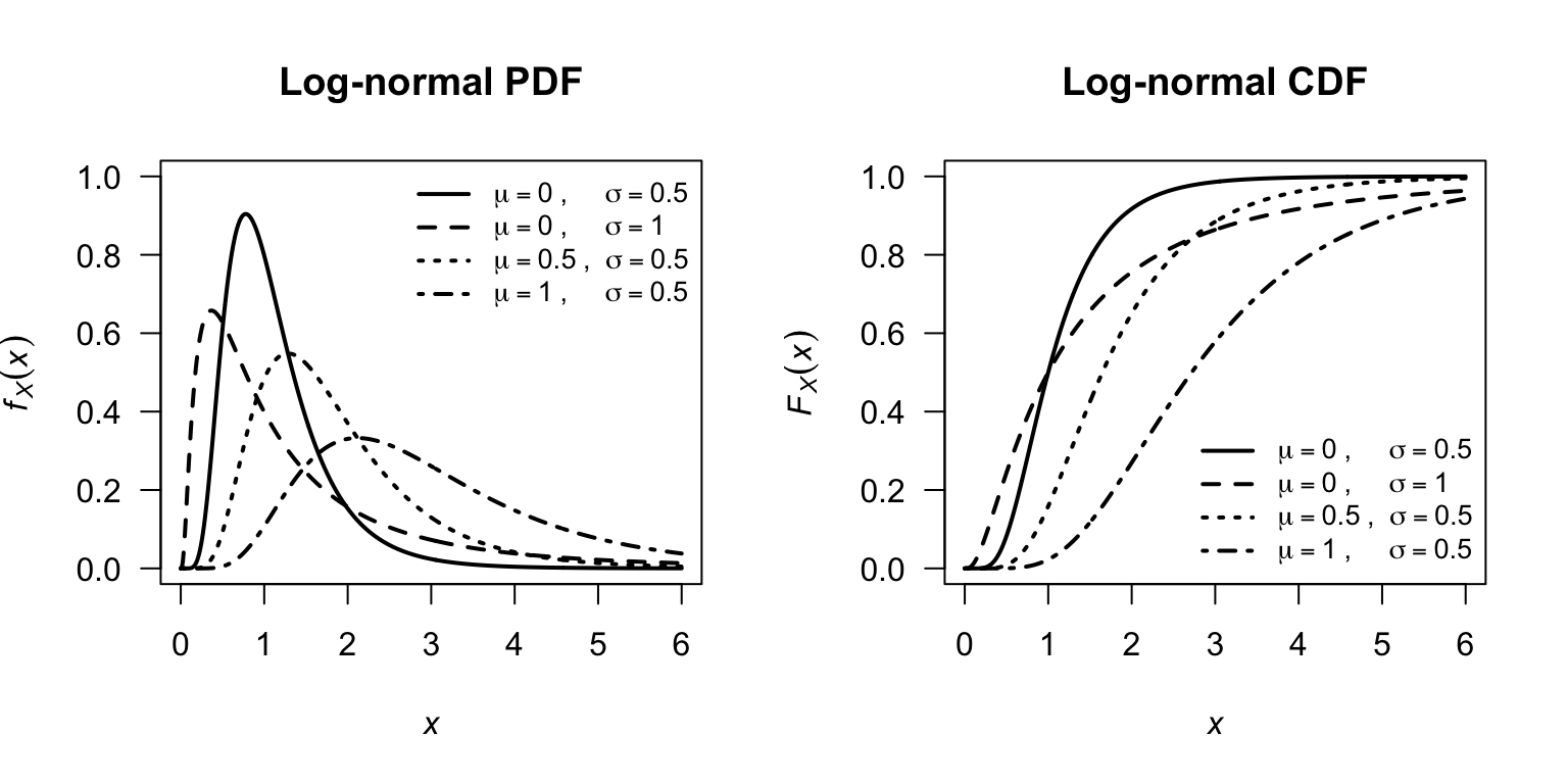
FIGURE 7.10: Log-normal PDFs (left) and CDFs (right) for selected parameter combinations.
7.6.2 Properties
The log-normal distribution has a heavier right tail than the normal, exponential, or gamma distributions for the same mean and variance. Its shape is always right-skewed (for \(\sigma > 0\)), becoming more symmetric as \(\sigma \to 0\).
Theorem 7.8 (Log-normal distribution properties) If \(X \sim \text{LogNormal}(\mu, \sigma^2)\) then
- \(\operatorname{E}[X] = \exp\!\left(\mu + \tfrac{1}{2}\sigma^2\right)\).
- \(\operatorname{var}[X] = \exp(2\mu + \sigma^2)\left[\exp(\sigma^2) - 1\right]\).
- The MGF of \(X\) does not exist for \(t > 0\).
- The median of \(X\) is \(\exp(\mu)\).
- The mode of \(X\) is \(\exp(\mu - \sigma^2)\).
Proof. Let \(Y = \log X \sim N(\mu, \sigma^2)\). For the expected value, write \(X = \exp Y\) and use the MGF of the normal distribution, \(M_Y(t) = \operatorname{E}[\exp(tY)] = \exp(\mu t + \sigma^2 t^2 / 2)\): \[ \operatorname{E}[X] = \operatorname{E}\left[\exp(Y)\right] = M_Y(1) = \exp\!\left(\mu + \tfrac{1}{2}\sigma^2\right). \] Similarly, \[ \operatorname{E}[X^2] = \operatorname{E}[\exp(2Y)] = M_Y(2) = \exp(2\mu + 2\sigma^2), \] and so \[\begin{align*} \operatorname{var}[X] &= \operatorname{E}[X^2] - \left(\operatorname{E}[X]\right)^2\\ &= \exp(2\mu + 2\sigma^2) - \exp(2\mu + \sigma^2)\\ &= \exp(2\mu + \sigma^2)\left[\exp(\sigma^2) - 1\right]. \end{align*}\] The median follows because \(\Pr(X \leq \exp\mu) = \Pr(Y \leq \mu) = 1/2\).
The MGF \(M_X(t) = \operatorname{E}[\exp(tX)]\) does not exist for \(t > 0\) because the log-normal has a sufficiently heavy right tail that \(\operatorname{E}[\exp(tX)] = \infty\) for all \(t > 0\): \(\exp(tX)\) grows faster than any polynomial in \(X\), and the log-normal tail is not light enough to control this growth.
Note that because the MGF does not exist, moments cannot be obtained by differentiating the MGF. Instead, the \(r\)-th raw moment follows directly from the normal MGF: \[ \operatorname{E}[X^r] = \operatorname{E}[\exp(rY)] = M_Y(r) = \exp\!\left(r\mu + \tfrac{1}{2}r^2\sigma^2\right). \]
A useful consequence is that the coefficient of variation \(\operatorname{CV}(X) = \sqrt{\operatorname{var}[X]}/\operatorname{E}[X]\) simplifies to \[ \operatorname{CV}(X) = \sqrt{\exp(\sigma^2) - 1}, \] which depends only on \(\sigma^2\), not on \(\mu\).
Example 7.13 (Income distribution) Income data are commonly modelled using a log-normal distribution (Aitchison 1957), since incomes are positive and right-skewed. Suppose annual household income \(X\) (in thousands of dollars) follows a \(\text{LogNormal}(\mu = 4, \sigma^2 = 0.25)\) distribution.
The income is: \[\begin{align*} \operatorname{E}[X] &= \exp\!\left(4 + \tfrac{1}{2}(0.25)\right) = \exp(4.125) \approx 61.9 \text{ (i.e., \$61,900)}.\\ \text{Median} &= \exp(4) \approx 54.6 \text{ (i.e., \$54,600)}. \end{align*}\] Note that the mean exceeds the median, reflecting the right skew.
The probability that a randomly selected household earns more than $100 000 is \(\Pr(X > 100) = \Pr(\log X > \log 100) = \Pr(Y > 4.605)\), where \(Y \sim N(4, 0.25)\): \[ \Pr(X > 100) = \Pr\!\left(Z > \frac{4.605 - 4}{0.5}\right) = \Pr(Z > 1.21) \approx 0.113. \] About \(11\)% of households earn more than $100,000.
Using R:
Example 7.14 (Transformation property) If \(X \sim \text{LogNormal}(\mu, \sigma^2)\), find the distribution of \(Y = X^k\) for some constant \(k \neq 0\).
Since \(X = \exp W\) where \(W \sim N(\mu, \sigma^2)\), we have \[ Y = X^k = \exp(kW). \] Now \(kW \sim N(k\mu,\, k^2\sigma^2)\), and since \(Y = \exp(kW)\) it follows that \[ Y \sim \text{LogNormal}(k\mu,\, k^2\sigma^2). \] In particular, \(1/X = X^{-1} \sim \text{LogNormal}(-\mu, \sigma^2)\). The log-normal family is closed under power transformations.
The log-normal and gamma distributions are both used for modelling positive random variables. The gamma distribution is best used when modelling a positive quantity formed by additive accumulation of many small contributions, such as rainfall amount in a day or total insurance claims over a period. The log-normal distribution is best used when modelling a positive quantity formed by multiplicative growth or compounding effects, such as income, wealth, or stock prices, where values arise from repeated proportional changes and can vary over orders of magnitude (i.e., with a long right tail).
7.7 Beta distribution
7.7.1 Definition
Some continuous random variables are constrained to a finite interval. The beta distribution is useful in these situations.
Definition 7.11 (Beta distribution) A random variable \(X\) with probability density function \[\begin{equation*} f_X(x; m, n) = \frac{x ^ {m - 1}(1 - x)^{n - 1}}{B(m, n)} \quad \text{for $0\leq x \leq 1$ and $m > 0$, $n > 0$}, \end{equation*}\] and \(B(m, n)\) is the beta function \[\begin{align} B(m, n) &= \int_0^1 x^{m - 1}(1 - x)^{n - 1} \, dx, \quad \text{for $m > 0$ and $n > 0$}\notag\\ &= \frac{\Gamma(m)\, \Gamma(n)}{\Gamma(m + n)}, \tag{7.13} \end{align}\] is said to have a beta distribution with parameters \(m\) and \(n\). We write \(X \sim \text{Beta}(m, n)\).
\(B(m, n)\) defined by (7.13) is known as the beta function with parameters \(m\) and \(n\). Since \(\int_0^1 f_X(x)\,dx = 1\) then \[ \int_0^1 \frac{x^{m - 1}(1 - x)^{n - 1}}{B(m, n)}\,dx = 1. \]
In R, the beta function is evaluated using beta(a, b), where a\({} = m\) and b\({} = n\).
The four R functions for working with the beta distribution have the form [dpqr]beta(., shape1, shape2) (see App. E):
-
dbeta(x, shape1, shape2)computes the PDF at \(X = {}\)x; -
pbeta(q, shape1, shape2)computes the CDF at \(X = {}\)q; -
qbeta(p, shape1, shape2)computes the quantile for cumulative probabilityp; and -
rbeta(n, shape1, shape2)generatesnrandom numbers,
where shape1\({}= m\) and shape2\({}= n\).
The distribution function for the beta distribution is complicated, involving incomplete beta functions, and will not be given.
Some properties of the beta function follow.
Theorem 7.9 (Beta function properties) The beta function in Eq. (7.13) satisfies the following:
- The beta function is symmetric in \(m\) and \(n\). That is, if \(m\) and \(n\) are interchanged, the function remains unaltered; i.e., \(B(m, n) = B (n, m)\).
- \(B(1, 1) = 1\).
- \(B\left(\frac{1}{2}, \frac{1}{2}\right) = \pi\).
Proof. To prove the first, put \(z = 1 - x\) and hence \(dz = -dx\) in Eq. (7.13). Then \[\begin{align*} B(m, n) &= -\int_1^0(1 - z)^{m - 1} z^{n - 1} \, dz\\ &= \int_0^1 z^{n - 1}(1 - z)^{m - 1} \, dz\\ &= B(n, m). \end{align*}\]
For the second, put \(x = \sin^2\theta\), and so \(dx = 2\sin\theta\cos\theta\,d\theta\), in Eq. (7.13). We have \[ B(m, n) = 2 \int_0^{\pi/2} \sin^{2m - 1}\theta \cos ^{2n - 1}\theta\,d\theta. \] So, for \(m = n = \frac{1}{2}\), \[ B\left(\frac{1}{2}, \frac{1}{2}\right) = 2\int_0^{\pi/2} d\theta = \pi. \]
For the third, note that \(\Gamma(1/2) = \sqrt{\pi}\) from Theorem 7.7. Further, since \(\Gamma(1) = 0! = 1\), the results follows.
Various gamma distributions are shown in the visualisation below, for different values of \(\alpha\) and \(\beta\).
FIGURE 7.11: Beta distributions.
When \(m = n = 1\), the beta distribution becomes the uniform distribution on \((0, 1)\).
7.7.2 Properties
Some basic properties of the beta distribution follow.
Theorem 7.10 (Beta distribution properties) If \(X \sim \text{Beta}(m, n)\) then
- \(\operatorname{E}[X] = m/(m + n)\).
- \(\displaystyle\operatorname{var}[X] = \frac{mn}{(m + n)^2 (m + n + 1)}\).
- A mode occurs at \(\displaystyle x = \frac{m - 1}{m + n - 2}\) for \(m, n > 1\).
Proof. Assume \(X \sim \text{Beta}(m, n)\), then \[\begin{align*} \mu_r' =\operatorname{E}[X^r] &= \int_0^1 \frac{x^r x^{m - 1}(1 - x)^{n - 1}} {B(m, n)}\,dx\\ &= \frac{B(m + r, n)}{B(m, n)} \int_0^1 \frac{x^{m + r - 1}(1 - x)^{n - 1}}{B(m + r, n)}\,dx\\ &= \frac{\Gamma(m + r)\,\Gamma(n)}{\Gamma(m + r + n)} \frac{\Gamma(m + n)}{\Gamma(m)\,\Gamma(n)}\\ &= \frac{\Gamma(m + r)\,\Gamma(m + n)}{\Gamma(m + r + n)\,\Gamma(m)} \end{align*}\] Putting \(r = 1\) and \(r = 2\) into the above expression, and using that \(\operatorname{var} = \operatorname{E}[X^2] - \operatorname{E}[X]^2\), the mean and variance are \[ \operatorname{E}[X] = m/(m + n) \quad \text{and} \quad \operatorname{var}[X] = \frac{mn}{(m + n)^2(m + n + 1)}. \] Any mode \(\theta\) of the distribution for which \(0 < \theta < 1\) will satisfy \(f'_X(\theta) = 0\). From the definition we see that for \(m, n>1\) and \(0 < x < 1\), \[ f'_X(x) = (m - 1)x^{m - 2} (1 - x)^{n - 1} - (n - 1)x^{m - 1}(1 - x)^{n - 1}/B(m, n) = 0 \] implying \((m - 1)(1 - x) = (n - 1)x\) which is satisfied by \(x = (m - 1) / (m + n - 2)\).
The MGF of the beta distribution cannot be written in terms of standard functions. The distribution function of the beta must be evaluated numerically in general, except when \(m\) and \(n\) are integers, as shown in the example below.
If \(X\sim \text{Beta}(m, n)\), then \(X\) is defined on \([0, 1]\). Sometimes then, the beta distribution is used to model proportions, though not proportions out of a total number (when the binomial distribution is used). Instead, the beta distribution is used, for example, to model percentage cloud cover (for instance, Falls (1974)).
For a random variable \(Y\) defined on a different closed interval \([a, b]\), define \(Y = X(b - a) + a\).
Example 7.15 Damgaard and Irvine (2019) use the beta-distribution to model the relative areas covered by plants of different species. The beta distribution is a suitable model, since these relative areas are proportions. In addition, the authors state (p. 2747) that
…plant cover data tend to be left-skewed (J-shaped), right skewed (L-shaped) or U-shaped
which align with some of the plots in Fig. 7.11.
Example 7.16 (Beta distributions) The bulk storage tanks of a fuel retailed are filled each Monday. The retailer has observed that over many weeks the proportion of the available fuel supply sold is well modelled by a beta distribution with \(m = 4\) and \(n = 2\).
If \(X\) denotes the proportion of the total supply sold in a given week, the mean proportion of fuel sold each week is \[ \operatorname{E}[X] = m/(m + n) = 4/6 = 2/3. \]
To find the probability that at least \(90\)% of the supply will sell in a given week, compute: \[\begin{align*} \Pr(X > 0.9) &= \int_{0.9}^1\frac{\Gamma(4 + 2)}{\Gamma(4)\Gamma(2)}x^3(1 - x)dx\\ &= 20\int_{0.9}^1 (x^3 - x^4))\,dx\\ &= 20(0.004)\\ &= 0.08 \end{align*}\] It is unlikely that \(90\)% of the supply will be sold in a given week. In R:
1 - pbeta(0.9,
          shape1 = 4,
          shape2 = 2)
#> [1] 0.08146
7.8 Other notable continuous distributions
The distributions discussed in this chapter are the mostly commonly used continuous distributions, but countless others exist. We mention a few.
Many commonly-used distributions are special cases of the gamma distribution. The Erlang distribution is a \(\text{Gamma}(k, 1/\lambda)\) distribution where = \(k\) is a positove integer, and arises as the sum of \(k\) independent exponential random variables. The Erlang distribution is often used in queuing theory. The chi-squared distribution (Sect. 12.7) with \(\nu\) degrees of freedom is a \(\text{Gamma}(\nu/2, 2)\) distribution, and appears often in statistics (see Chap. 12.4).
The Weibull distribution is defined on \([0, \infty)\) (which includes zero) and is used to model lifetimes and failures, and is used in reliability analysis and survival analysis.
The Pareto distribution is defined on \((x_m, \infty)\) for some minimum value \(x_m > 0\), and has a heavy right tail; it is used to model income distributions, insurance losses, and other phenomena where extreme values are more common than a normal or exponential distribution would suggest.
The Cauchy distribution is defined on the entire real-line, but has heavier tails than the normal distribution. It is used to model the ratio of two independent normal variables.
The von Mises distribution is defined on \([-\pi, \pi)\) and is used to model angles; it is sometimes called the ‘circular normal distribution’. It is used to model wind directions and animal movements.
The arcsine distribution is a special case of the beta distribution and is hence defined on \((0, 1)\), with probability concentrated near the limits of the range at \(x = 0\) and \(x = 1\). It arises in the study of random walks and Brownian motion.
Several other continuous distributions emerge when studying sampling (Chap. 12.4), and are usually related to the normal distribution. The \(t\)-distribution (Sect. 12.8) is similar to a normal distribution (and defined on the entire real line) but with heavier tails, and is fundamental to statistical inference about means. The \(F\)-distribution (Sect. 12.9), defined on \((0, \infty)\), is related to the ratio of independent \(\chi^2\) distributions, and is fundamental for analysis variance.
7.9 Simulation
7.9.1 Simulating continuous distributions
As with discrete distributions (Sect. 6.10), simulation can be used with continuous distributions.
Again, in R, random numbers from a specific distribution use functions that start with the letter r (see Sect. E for details for specific distributions); for example:
###   Random numbers from normal, mean = 4 and sd = 2
rnorm(10,               # Generate 10 random numbers...
      mean = 4,         # ... with mean = 4
      sd = 2)           # ... with sd = 2
#>  [1] 1.748524 4.082457 2.624341 4.104625 6.415505 7.795946
#>  [7] 3.036380 3.385202 8.079291 6.638584


###   Random numbers from beta, shape1 = 1.4 and shape2 = 0.5
rbeta(10,               # Generate 10 random numbers...
      shape1 = 1.4,     # ... with m = 1.4
      shape2 = 0.5)     # ... and n = 0.5
#>  [1] 0.82779655 0.84502692 0.97464210 0.03513962 0.95732546
#>  [6] 0.66385037 0.93865839 0.45304821 0.93295216 0.54553409
Random numbers from discrete and continuous distributions can be used together to model and understand many phenomena.
7.9.2 Example: relationships between distributions
Relationships commonly exist between distributions. For example, the gamma distribution is related to the exponential distribution. If a random variable \(X\) has an exponential distribution with rate parameter \(\lambda\), then the distribution of \[ Y = \sum_{i = 1}^k X \] has a gamma distribution, with shape parameter \(\alpha = k\) and rate parameter \(\lambda\). This can be shown using simulation (Fig. 7.12):
set.seed(67433)
### An exponential variate with  rate = 2
X <- rexp(n = 5000,
          rate = 3)
Y <- matrix( data = X,
             ncol = 5, # Place 5 values in each of 1000 rows
             nrow = 1000)
Y <- rowSums(Y) # Sum five values in each row
The histograms of \(X\) and \(Y\) can then be shown:
### Set up for two plots, side-by-side
par(mfrow = c(1, 2) )

### Plot two histograms: Y and X
hist(X,
     freq = FALSE,
     las = 1,
     main = "Exponential density",
     xlab = expression(italic(x) ),
     ylab = "Density")
hist(Y,
     freq = FALSE,
     las = 1,
     ylim = c(0, 0.6),
     main = "Gamma density",
     xlab = expression(italic(y) ),
     ylab = "Density")

### Now overlay  the theoretical gamma distribution
# dgamma()  is the density function for a gamma distribution
curve(dgamma(x, shape = 5, rate = 3),
      from = 0,
      to = 10,
      lwd = 3,    # Thicker lines
      add = TRUE) # Add to existing plot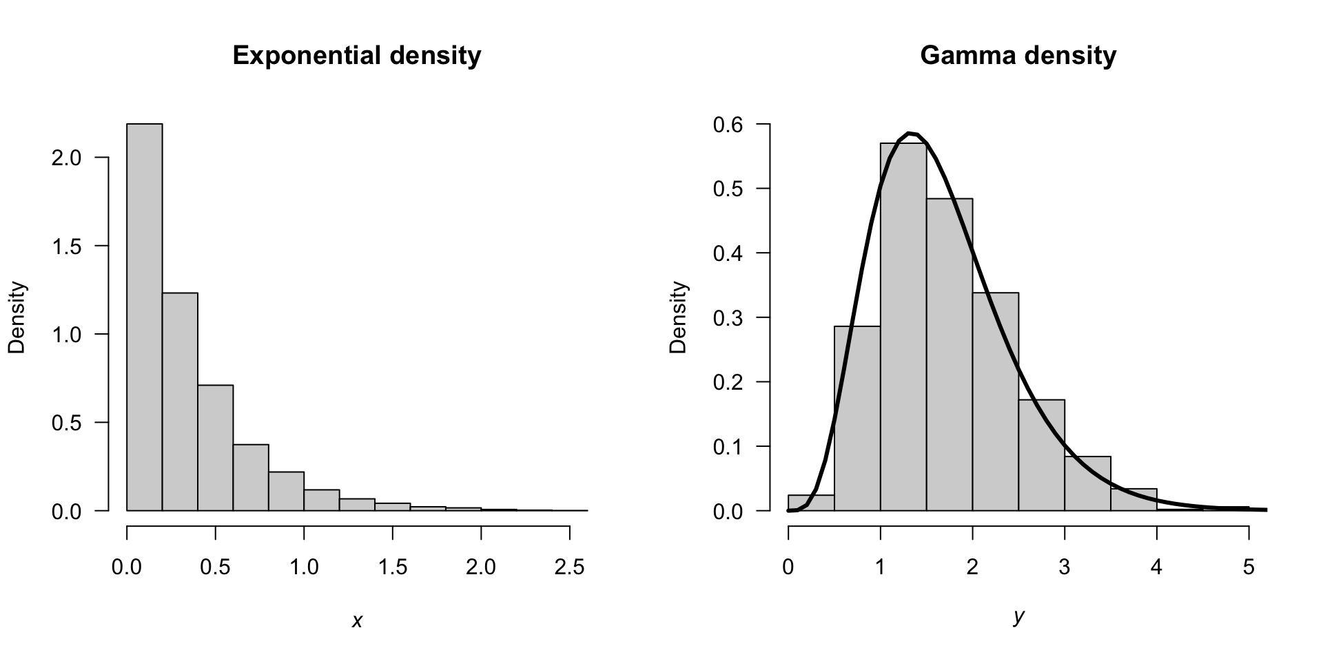
FIGURE 7.12: Left: histogram of \(5000\) simulated values from an exponential distribution. Right: histogram of the sum of five independent exponential distributions. The solid lines on the right panel is the theoretical distribution of a gamma distribution with a shape parameter of \(5\).
7.9.3 Example: heights
Suppose we are seeking women over \(173\,\text{cm}\) tall for a study; what percentage of women are over \(173\,\text{cm}\) tall? Assume that adult females have heights modelled by a normal distribution with mean \(163\,\text{cm}\) and a standard deviation of \(5\,\text{cm}\) (Australian Bureau of Statistics 1995). The percentage taller than \(173\,\text{cm}\) is:
1 - pnorm(173,
          mean = 163,
          sd = 5)
#> [1] 0.02275013
Simulations can also be used, which allows us to consider more complex situations. For this simple question initially (Fig. 7.13, left panel):
htW <- rnorm(1000,  # One thousand women
             mean = 163,  # Mean ht
             sd = 5)      # Sd of height
pcTallWomen <- sum( htW > 173 )/1000 * 100

cat("Percentage 'tall' women:", pcTallWomen, '%\n')
#> Percentage 'tall' women: 2.3 %
Now consider a more complex situation. Suppose adult males have heights with a mean of \(175\,\text{cm}\) with standard deviation of \(7\,\text{cm}\), and constitute \(46\)% of the population. Now, we are seeking women or men over \(173\,\text{cm}\) tall (Fig. 7.13, right panel):
personSex <- rbinom(1000,  # Select sex of each person
                    1,
                    0.46) # So 0 = Female; 1 = Male

htP <- rnorm(1000,  # change ht parameters according to sex
             mean = ifelse(personSex == 1,
                           175,
                           163),
             sd = ifelse(personSex == 1,
                         7,
                         5))

pcTallPeople <- sum( htP > 173 )/1000 * 100
pcFemales <- sum( personSex == 0 ) / 1000 * 100

cat("Percentage 'tall' people:", pcTallPeople, "\n",
    "Percentage females:", pcFemales, "\n",
    "Percentage of 'tall' people that are female:",
       round( sum(htP > 173 & personSex == 0) / sum(htP > 173) * 100, 1), "\n",
    "Variance of heights: ", var(htP), "\n")
#> Percentage 'tall' people: 29.9
#>  Percentage females: 54.1
#>  Percentage of 'tall' people that are female: 4
#>  Variance of heights:  75.77411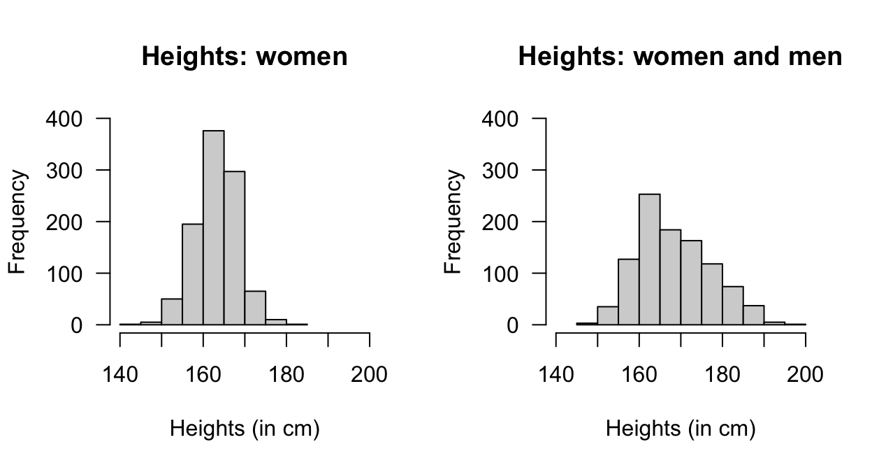
FIGURE 7.13: The empirical probability density function of heights of women (left panel) and men and women combined (right panel).
7.9.4 Example: simulating patient recovery times
A hospital is studying patient recovery times after a surgical procedure. Three quantities are of interest:
- The recovery time \(T\) (in days) until a patient is discharged. \(T\) is modelled as \(T \sim \text{Exp}(\beta = 5)\) (i.e., the mean recovery time is \(5\) days).
- The pain score \(P\) (on a continuous \(0\)–\(10\) scale) at discharge. \(P\) is modelled as \(P \sim \text{Beta}(\alpha = 2, \beta = 4)\), rescaled to the interval \([0, 10]\) (with a mean score of \(2/(2 + 4) \times 10 = 3.33\)).
- Whether the patient is readmitted within \(30\) days \(B\). \(B\) is modelled as a \(\text{Bernoulli}(p = 0.15)\) random variable.
We can use R to simulate \(n = 10\,000\) patients:
n         <- 10000                      # Number of simulations
recovery  <- rexp(n, rate = 1/5)        # Exp(scale = 5)
pain <- rbeta(n, shape1 = 2, shape2 = 4) * 10
readmit   <- rbinom(n,
                    size = 1,
                    prob = 0.15)
The simulated summaries can be compared to their theoretical values:
cat("--- Recovery time ---\n",
    "Theoretical mean:    ", 5, "\n",
    "Simulated mean:      ", round(mean(recovery), 2), "\n\n")
#> --- Recovery time ---
#>  Theoretical mean:     5
#>  Simulated mean:       4.98

cat("--- Pain score ---\n",
    "Theoretical mean:    ", round(2/(2 + 4) * 10, 2), "\n",
    "Simulated mean:      ", round(mean(pain), 2), "\n",
    "Simulated sd:        ", round(sd(pain), 2), "\n")
#> --- Pain score ---
#>  Theoretical mean:     3.33
#>  Simulated mean:       3.32
#>  Simulated sd:         1.79

cat("--- Readmission ---\n",
    "Theoretical rate:    ", 0.15, "\n",
    "Simulated rate:      ", round(mean(readmit), 3), "\n\n")
#> --- Readmission ---
#>  Theoretical rate:     0.15
#>  Simulated rate:       0.152
What proportion of patients have a recovery time exceeding \(7\) days? We can answer this both analytically and via simulation:
cat("Theoretical P(T > 7):",
    round(1 - pexp(7, rate = 1/5), 3), "\n",
    "Simulated P(T > 7):  ",
    round(mean(recovery > 7), 3), "\n")
#> Theoretical P(T > 7): 0.247
#>  Simulated P(T > 7):   0.245
Now consider some complex questions that would be difficult to answer analytically. Suppose we are interested in the mean recovery time for patients who are readmitted. This is a conditional expectation, and is straightforward to estimate from simulation:
cat("Mean recovery time, readmitted patients:    ",
    round(mean(recovery[readmit == 1]), 2), "\n",
    "Mean recovery time, non-readmitted patients:",
    round(mean(recovery[readmit == 0]), 2), "\n")
#> Mean recovery time, readmitted patients:     4.81
#>  Mean recovery time, non-readmitted patients: 5.01
Suppose we are interested in the probability that a patient has both a long recovery (\(T > 7\)) and a high pain score (\(P > 6\)):
cat("P(T > 7 and P > 6):",
    round(mean(recovery > 7 & pain > 6), 3), "\n")
#> P(T > 7 and P > 6): 0.02
If \(T\) and \(P\) were independent, we would expect this probability to be approximately:
cat("P(T > 7) x P(P > 6):",
    round(mean(recovery > 7) * mean(pain > 6), 3), "\n")
#> P(T > 7) x P(P > 6): 0.022
Since \(T\) and \(P\) were simulated independently, these are close (as expected).
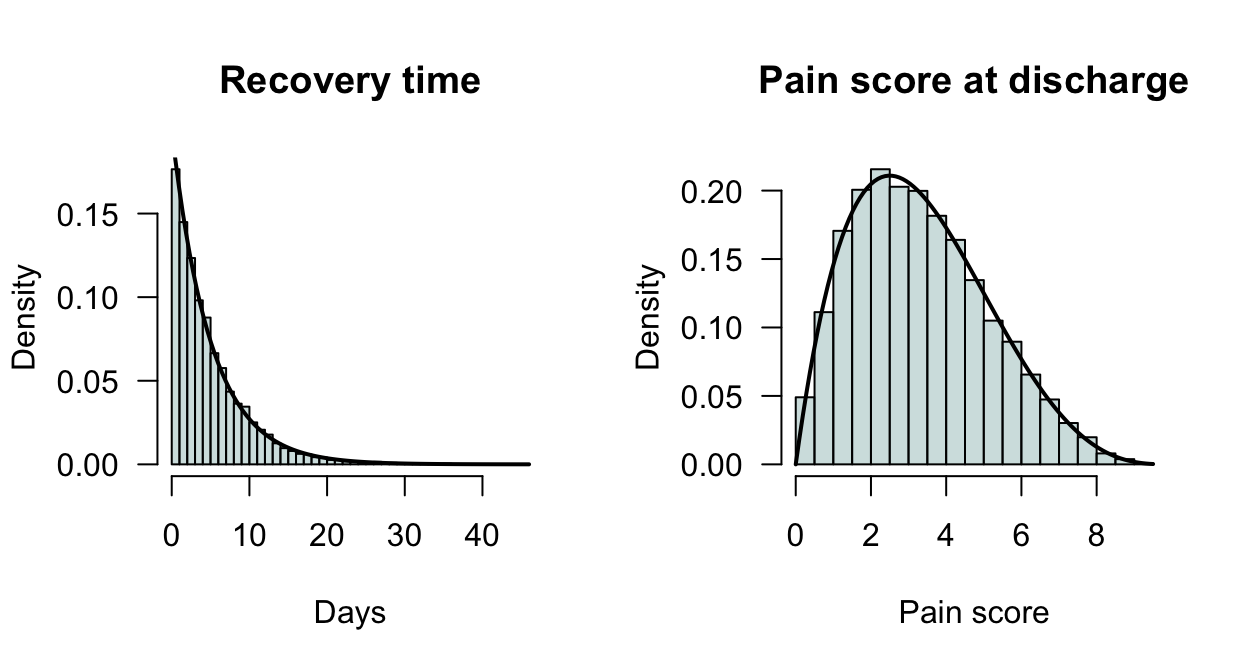
FIGURE 7.14: The empirical probability density function of simulated recovery times (left) and pain scores at discharge (right). The theoretical exponential density is overlaid on the left panel.
We may also wish to know the mean recovery time given high pain and readmission, \(\operatorname{E}[T\mid P > 6, \text{readmitted}]\). Conditioning on two things simultaneously is analytically messy but trivial in simulation:
cat("Mean recovery time (high pain + readmitted):",
    round(mean(recovery[pain > 6 & readmit == 1]), 2), "\n")
#> Mean recovery time (high pain + readmitted): 4.27
Finally, we may ask: What is the probability total bed usage exceeds \(70\) days?
n_wards <- 10000
total_beds <- replicate(n_wards, {
  sum(rexp(10, rate = 1/5))
})
cat("P(total bed-days > 70):",
    round(mean(total_beds > 70), 3), "\n",
    # Analytically: total ~ Gamma(10, 5), so verify:
    "Theoretical P(total > 70):",
    round(1 - pgamma(70, shape = 10, scale = 5), 3), "\n")
#> P(total bed-days > 70): 0.112
#>  Theoretical P(total > 70): 0.109
7.10 Exercises
Selected answers appear in Sect. F.6.
Exercise 7.1 For each scenario, choose the most appropriate distribution from: Continuous uniform, Normal, Exponential, Gamma, Lognormal, Beta. Briefly justify your choice.
- The proportion of time a server is busy during a randomly selected hour.
- The lifetime of an electronic component until it fails, assuming a constant failure rate.
- The amount of time a customer spends in a queue before being served.
Exercise 7.2 For each scenario, choose the most appropriate distribution from: Continuous uniform, Normal, Exponential, Gamma, Lognormal, Beta. Briefly justify your choice.
- The distribution of adult IQ scores in a large population.
- The time until a website receives its 100th visit.
- The size of a randomly selected insurance claim.
Exercise 7.3 Choose the most appropriate distribution from: Continuous uniform, Normal, Exponential, Gamma, Lognormal, Beta. Briefly justify your choice.
- The proportion of time a machine is operational during a randomly selected shift.
- The total time spent waiting for 3 consecutive service completions in a call centre.
- The daily percentage change in a stock price (assumed symmetric around 0 for small movements).
Exercise 7.4 Choose the most appropriate distribution from: Continuous uniform, Normal, Exponential, Gamma, Lognormal, Beta. Briefly justify your choice.
- The time between two consecutive earthquakes in a region where earthquakes occur randomly at a constant average rate.
- The file size (MB) of a randomly selected file on a server.
- The concentration of a pollutant measured across many sites, where values vary due to multiplicative environmental factors.
Exercise 7.5 Suppose \(X\sim \text{Unif}(-5, 5)\) is a continuous random variable.
- Find \(\Pr(X > 3)\).
- Find \(\Pr(X > 3 \mid X > 0)\).
- Find \(\Pr(|X| > 3)\).
- Find \(\Pr\big( (X > 3) \cup (X > 0)\big)\).
- Find \(\Pr\big( (X > 3) \cap (X > 0)\big)\).
- Find and plot the distribution function of \(X\).
- What is the probability that two random values of \(X\) are both larger than \(0\)?
Exercise 7.6 Suppose \(T\sim \text{Unif}(20, 40)\) is a continuous random variable.
- Find \(\Pr(T < 33)\).
- Find \(\Pr(T > 30 \mid T > 25)\).
- Find \(\Pr(|T - 30| < 5)\).
- Find \(\Pr\big( (T > 30) \cup (T > 25)\big)\).
- Find \(\Pr\big( (T > 30) \cap (T > 25)\big)\).
- Find and plot the distribution function of \(T\).
- What is the probability that neither of two random values of \(T\) are larger than \(35\)?
Exercise 7.7 Suppose that the measured voltage in a certain electrical circuit has a normal distribution with mean \(120\,\text{V}\) and standard deviation \(2\,\text{V}\).
- What is the probability that a measurement will be between \(116\) and \(118\,\text{V}\)?
- What is the probability that a measurement will be between \(120\) and \(125\,\text{V}\)?
- What is the probability that a measurement will be between \(115\) and \(120\,\text{V}\)?
- What is the probability that a measurement will be larger than \(118\,\text{V}\)?
- What is the probability that a measurement will be smaller than \(118\,\text{V}\)?
- What is the probability that a measurement will be smaller than \(123\,\text{V}\)?
- What is the probability that a measurement will be smaller than \(101\,\text{V}\)?
- Ten percent of measurements will be less than what voltage?
- Sixty percent of measurements will be less more than what voltage?
- If five independent measurements of the voltage are made, what is the probability that three of the five measurements will be between \(116\) and \(118\,\text{V}\)?
Exercise 7.8 Suppose that the volume of hot water dispensed by a coffee machine has a normal distribution with mean \(170\,\text{mL}\) and standard deviation \(3\,\text{mL}\).
- What is the probability that between \(165\) and \(175\,\text{mL}\) will be dispensed?
- What is the probability that more than \(172\,\text{mL}\) will be dispensed?
- What is the probability that between \(165\,\text{mL}\) will be dispensed?
- What is the probability that more than \(185\,\text{mL}\) will be dispensed?
- What is the probability that more than \(160\,\text{mL}\) will be dispensed?
- What is the probability that more than \(170\,\text{mL}\) will be dispensed?
- Twenty percent of cups will be dispensed with less than what amount of hot water?
- Thirty percent of cups will be dispensed with more than what amount of hot water?
- If six cups of coffee are made independently, what is the probability that exactly three cups will contain more than \(175\,\text{mL}\)?
Exercise 7.9 At a large call centre, the time between the arrival of phone calls are independent and exponentially distributed with a mean of \(4\,\text{mins}\).
- Determine the probability that time between phone calls is less than \(2\,\text{mins}\).
- Determine the probability that time between phone calls is more than \(10\,\text{mins}\).
- Determine the probability that time between phone calls is between \(2\,\text{mins}\) and \(5\,\text{mins}\).
- Fifteen percent of intervals between phone calls are less than what time?
- Thirty percent of intervals between phone calls are more than what time?
Exercise 7.10 A company buys a large number of identical components, whose failure times are independent and exponentially distributed with mean \(100\,\text{h}\).
- Determine the probability that one component will survive for less than \(80\,\text{h}\).
- Determine the probability that one component will survive between \(150\,\text{h}\) and \(200\,\text{h}\).
- Determine the probability that one component will survive at least \(150\,\text{h}\).
- Determine the probability that one component will survive for more than \(150\,\text{h}\).
- Ten percent of components will last longer than how long?
- Twenty-five percent of components will fail before what lifetime?
- What is the probability that at least \(125\) out of \(500\) components will survive at least \(150\,\text{h}\)?
Exercise 7.11 GAMMA: Monthly rainfall at a certain station is modelled as \(\text{Gamma}()\) distribution.
Exercise 7.12 GAMMA: Daily wind energy production (in kWh) at a wind farm is modelled as \(\text{Gamma}()\) distribution.
Exercise 7.13 LOG-NORMAL: Let \(X\) be the total duration of rainfall during a storm event.
Exercise 7.14 LOG-NORMAL: Let X be the file size (in MB) of a randomly chosen file on a server.
Exercise 7.15 For each scenario, decide whether a Gamma or Lognormal distribution is more appropriate for modelling the random variable. Briefly justify your answer.
- The daily amount of rainfall (mm) at a weather station.
- The income of individuals in a large population.
- The total annual cost of insurance claims for a policyholder.
Answer 1 Gamma — rainfall is an accumulated quantity over time, formed by many small additive contributions (rain events). Lognormal — income is generated through multiplicative effects (education, experience, industry, growth), producing strong right skew. Gamma — insurance claim totals are sums of many individual claims, an additive accumulation process.
Exercise 7.16 For each scenario, decide whether a Gamma or Lognormal distribution is more appropriate for modelling the random variable. Briefly justify your answer.
- The file size (MB) of a randomly selected file stored on a server.
- The total time spent servicing requests at a help desk in one day.
- The price of a stock at a fixed future time.
Answer 2 Lognormal — file sizes arise from multiplicative processes (compression, content generation, scaling), leading to wide variation and heavy right tail. Gamma — total service time is an accumulation of many small service durations (additive waiting/processing times). Lognormal — stock prices evolve through multiplicative returns (compounded growth), producing a skewed positive distribution.
Exercise 7.17 In a given city, the proportion of cloud cover at 5pm on a randomly selected day follows a Beta\((m=3, n=4)\) distribution.
- Find the mean proportion of cloud cover at 5pm.
- Find the probability that the cloud cover exceeds \(60\)% at 5pm.
- Find the probability that the cloud cover is less than \(25\)% at 5pm.
- Find the probability that the cloud cover is between \(30\)% and \(50\)% at 5pm.
- Ninety percent of days have less than what cloud cover proportion?
- Eighty percent of days have more than what cloud cover proportion?
Exercise 7.18 Let \(X\) be the proportion of time that a machine operates during a randomly selected \(8\)-hour shift. Suppose \(X\sim\text{Beta}(m=13, n=2)\).
- Find the mean proportion of time that the machine is operating during an \(8\)-hr shift.
- Find the probability that the machine operates for more than \(90\)% of an \(8\)-hr shift.
- Find the probability that the machine operates for less than \(75\)% of an \(8\)-hr shift.
- Find \(\Pr(X > 95 \mid X > 90)\).
- Find the \(60\)th percentile of \(X\).
- Find the \(35\)th percentile of \(X\).
Exercise 7.19 Write the beta distribution parameters \(m\) and \(n\) in terms of the mean and variance.
Exercise 7.20 In a study modelling pedestrian road-crossing behaviour (Shaaban and Abdel-Warith 2017), the uniform distribution is used in the simulation to model the vehicle speeds. The speeds have a minimum value of \(30\) km.h\(-1\), and a maximum value of \(72\) km.h\(-1\).
- Using this model, compute the mean and standard deviation of vehicle speeds.
- Compute and plot the PDF and distribution function.
- If \(X\) is the vehicle speed, compute \(\Pr(X > 60)\), where \(60\) km.h\(-1\) is the posted speed limit.
- Compute \(\Pr(X > 65\mid X > 60)\).
Exercise 7.21 In a study modelling pedestrian road-crossing behaviour (Shaaban and Abdel-Warith 2017), the normal distribution is used in the simulation to model the vehicle speeds. The normal model has a mean of \(48\) km/h, with a standard deviation2 of \(8.8\) km.h\(-1\).
- The article ignores all vehicles travelling slower than \(30\) km.h\(-1\) and faster than \(72\) km.h\(-1\). What proportion of vehicles are excluded using this criterion?
- Write the PDF for this truncated normal distribution.
- Plot the PDF and df for this truncated normal distribution.
- Compute the mean and variance for this truncated normal distribution.
- Suppose a vehicle is caught speeding (i.e., exceeding \(60\) km.h\(-1\)); what is the probability that the vehicle is exceeding the speed limit by less than \(5\) km.h\(-1\)?
Exercise 7.22 Show that the mode of a log-normal distribution is \(x^* = \exp(\mu - \sigma^2)\).
Exercise 7.23 Show that the exponential probability density function is monotonically decreasing over \(\mathbb{R}+\).
Exercise 7.24 A study of the service life of concrete in various conditions (Liu and Shi 2012) modelled the diffusion coefficients using a gamma distribution, with \(\alpha = 27.05\) and \(\beta = 1.42\) (unitless).
- Plot the PDF and df.
- Determine the mean and standard deviation of the chloride diffusion coefficients that were used in the simulation.
- If \(C\) represents the chloride diffusion coefficients, compute \(\Pr(C > 30\mid C < 50)\).
Exercise 7.25 A study of the service life of concrete in various conditions (Liu and Shi 2012) used normal distributions to model the surface chloride concentrations. In one model, the mean was set as \(\mu = 2\) kg.m\(-3\) and the standard deviation as \(\sigma = 0.2\) kg.m\(-3\).
- Plot the PDF and df.
- Let \(Y\) be the surface chloride concentration. Compute \(\Pr(Y > 2.4)\).
- \(80\)% of the time, surface chloride concentrations are below what value?
- \(15\)% of the time, surface chloride concentrations exceed what value?
Exercise 7.26 An alternative to the beta distribution with a closed form is the Kumaraswamy distribution, with PDF \[ p_X(x) = ab x^{a - 1} (1 - x^a)^{b - 1} \qquad \text{for $0 < x < 1$} \] for \(a > 0\) and \(b > 0\). We write \(X\sim \text{Kumaraswamy}(a, b)\).
- Plot some densities for the Kumaraswamy distribution showing its different shapes.
- Show that the df is \(F_X(x) = 1 - (1 - x^a)^b\) for \(0 < x < 1\). Plot the distribution functions corresponding to the PDFs in Part 1.
- If \(X\sim \text{Kumaraswamy}(a, 1)\), then show that \(X\sim \text{Beta}(a, 1)\).
- If \(X\sim \text{Kumaraswamy}(1, 1)\), then show that \(X\sim \text{Unif}(0, 1)\).
- If \(X\sim \text{Kumaraswamy}(a, 1)\), then show that \((1 - X) \sim \text{Kumaraswamy}(1, a)\).
Exercise 7.27 Show that the gamma distribution has a constant coefficient of variation, where the coefficient of variation is the standard deviation divided by the mean.
Exercise 7.28 In a study modelling waiting times at a hospital (Khadem et al. 2008), patients are classified into one of three categories: Red (critically ill or injured patients), Yellow (moderately ill or injured patients), or Green (injured or uninjured patients).
For ‘Green’ patients, the service time \(S\) was modelled as \(S = 4.5 + 11V\), where \(V \sim \text{Beta}(0.287, 0.926)\).
- Find the mean and standard deviation of the service times \(S\).
- Produce well-labelled plots of the PDF and distribution function of \(V\), showing important features.
Exercise 7.29 In a study modelling waiting times at a hospital (Khadem et al. 2008), patients are classified into one of three categories: Red (critically ill or injured patients), Yellow (moderately ill or injured patients), or Green (injured or uninjured patients).
The time (in minutes) spent in the reception are for Yellow patients, say \(T\), is modelled as \(T = 0.5 + W\), where \(W\sim \text{Exp}(\beta = 16.5)\).
- Find the mean and standard deviation of the waiting times \(T\).
- Plot the PDF and distribution function of \(W\).
- Determine \(\Pr(T > 1)\).
Exercise 7.30 In a study modelling waiting times at a hospital (Khadem et al. 2008), patients are classified into one of three categories: Red (critically ill or injured patients), Yellow (moderately ill or injured patients), or Green (injured or uninjured patients).
The time (in minutes) spent in the reception are for Green patients, say \(T\), is modelled as a normal with mean \(\mu = 45.4\,\text{mins}\) and standard deviation \(\sigma = 23.4\,\text{mins}\).
- Find the mean and standard deviation of the waiting times \(T\).
- Plot the PDF and distribution function of \(T\).
- What proportion of ‘Green’ patients wait longer than an hour?
- How long to the slowest \(10\)% of patients need to wait?
Exercise 7.31 In a study of rainfall (Watterson and Dix 2003), rainfall on wet days in SE Australia (37\(\circ\)S; 146\(\circ\)E) was simulated using a gamma distribution with \(\alpha = 0.62\) and \(\beta = 7.1\)mm.
- Rainfall below \(0.0017\,\text{mm}\) cannot be recorded by the equipment used. What proportion of days does this represent?
- Plot the PDF and df.
- What is the probability that more than \(3\,\text{mm}\) falls on a wet day?
- The proportion of wet days is \(0.43\). What proportion of all days receive more than \(3\,\text{mm}\)?
Exercise 7.32 In a study of rainfall disaggregation (Connolly et al. 1998) (extracting small-scale rainfall features from large-scale measurements), the duration (in fractions of day) of non-overlapping rainfall events per day at Katherine was modelled using a Gamma distribution with \(\alpha = 2\), and \(\beta = 0.04\) in summer and \(\beta = 0.03\) in winter.
Denote the duration of rainfall events, in fractions of a day, be denoted in summer as \(S\), and in winter as \(W\).
- Plot the rainfall event duration distributions, and compare summer and winter.
- What is the probability of a rainfall event lasting more than \(6\,\text{h}\) in winter?
- What is the probability of a rainfall event lasting more than \(6\,\text{h}\) in summer?
- Describe what is meant by the statement \(\Pr(S > 3/24 \mid S > 1/24)\), and compute the probability.
- Describe what is meant by the statement \(\Pr(W < 2/24 \mid W > 1/24)\), and compute the probability.
Exercise 7.33 In a study of rainfall disaggregation (Connolly et al. 1998) (extracting small-scale rainfall features from large-scale measurements), the starting time of the first rainfall event at Katherine each day (scaled from 0 to 1) was modelled using a beta distribution with parameters \((1.16, 1.50)\) in summer and \((0.44, 0.56)\) in winter.
Denote the number of rainfall events in summer as \(S\), and in winter as \(W\).
- Plot the two starting-time distributions, and compare summer and winter.
- Compute the mean and standard deviation of starting times for both seasons.
- What is the probability that the first rain event in winter is after 6am?
- What is the probability that the first rain event in summer is after 6am?
- Describe what is meant by the statement \(\Pr(S > 3 \mid S > 1)\), and compute the probability.
- Describe what is meant by the statement \(\Pr(W > 2 \mid W > 1)\), and compute the probability.
Exercise 7.34 A study of the impact of diarrhoea (Schmidt et al. 2009) used a gamma distribution to model the duration of symptoms. In Guatemala, duration (in days) was modelled using a gamma distribution with \(\alpha = 1.11\) and \(\beta = 3.39\). Let \(X\) refer to the duration of symptoms.
- Compute the mean and standard deviation of the duration.
- The value of \(\alpha\) is close to one. Plot the PDF of the gamma distribution and the near-equivalent exponential distribution, and comment.
- Compute \(\Pr(X > 4)\) using both the gamma and exponential distributions, and comment.
- The patients in the \(5\)% with symptoms the longest had symptoms for how long? Again, compare both models, and comment.
Exercise 7.35 In a study of office occupancy at a university (Luo et al. 2017), the leaving-times of professors were modelled as a normal distribution, with a mean leaving time of 6pm, with a standard deviation of \(1.5\,\text{h}\).
- Using this model, what proportion of professors leave before 5pm?
- Suppose a professor is still at work at 5pm; what is the probability that the professor leaves after 7pm?
- The latest-leaving \(15\)% of professors leave after what time?
Exercise 7.36 The percentage of clay content in soil has been modelled using a beta distribution. In one study (Haskett et al. 1995), two counties in Iowa were modelled with beta-distributions: County A with parameters \(m = 11.52\) and \(n = 4.75\), and County B with parameters \(m = 3.85\) and \(n = 3.65\).
- Plot the two distributions, and comment (in context).
- Compute the mean and standard deviation of each county.
- What percentage of soil samples exceed \(50\)% clay in the two counties? Comment.
Exercise 7.37 A study of water uptake in plants in grasssland and savanna ecosystems (Nippert and Holdo 2015) used a beta distribution to model the distribution of root depth \(D\). The MRD (maximum root density) was \(70\,\text{cm}\), so the beta distribution used was defined over the interval \([0, 70]\). For one simulation, the beta-distribution parameters were \(m = 1\) and \(n = 5\).
- Plot the PDF, and explain what it means in this context.
- Determine the probability that the root depth was deeper than \(50\,\text{cm}\).
- Determine the root depth of the plants with the deepest \(20\)% of roots.
Exercise 7.38 A headway is the time gap (front-bumper to front-bumper) separating consecutive motor vehicles in a lane of road traffic. Suppose headways \(X\) (in seconds) on a section of a traffic lane are described by a shifted gamma distribution, with PDF \[ f_X(x) = \frac{1}{\beta^\alpha \Gamma(\alpha)} (x - \Delta)^{\alpha - 1} \exp\left( -(x - \Delta)/\beta\right) \quad\text{for $x > \Delta$}, \] where \(\alpha = 2.5\), \(\beta = 0.8\) and \(\Delta = 1.2\).
- Determine the theoretical mean and variance of this distribution.
- Simulate \(1000\) headways using R, and plot a histogram of the data. Comment.
- Using the simulation results, estimate the probability that a headway is within two standard deviations of the mean.
- Confirm that Tchebyshev’s inequality holds for the above probability.
Exercise 7.39 Another commonly-used distribution is the Weibull distribution: \[ f_Y(y) = \frac{k}{\lambda} \left( \frac{x}{\lambda} \right)^{k - 1} \exp( -(x/\lambda)^k)\quad\text{for $x > 0$}, \] where \(\lambda > 0\) is called a scale parameter, and \(k > 0\) is called a shape parameter.
- Produce some sketches in R to show the variety on the shapes of the density function.
- Derive the mean and variance of the Weibull distribution.
- Derive the cdf for the Weibull distribution.
Exercise 7.40 Raschke (2011) modelled the humidity at the Haarweg Wageningen (Netherlands) weather station in May 2007 and 2008 using beta distributions. In May 2007, the relative humidity was modelled with a \(\text{Beta}(6.356, 1.970)\) distribution; in May 2008, with the \(\text{Beta}(2.803, 1.456)\) distribution.
- With the given models, determine the mean and variance of the humidity for both months.
- On the same graph, plot both distributions, and comment.
- For May 2008, compute \(\Pr(X > 60)\), where \(X\) is the relative humidity, based on the model.
- For May 2008, compute \(\Pr(X > 60 \mid X > 50)\), where \(X\) is the relative humidity, based on the model.
- For May 2008, \(80\)% of days have a relative humidity less than what value, based on the model?
Exercise 7.41 Based on Pfizer Australia (2008), the mean height \(Y\) of Australian girls aged between \(2\) and \(5\) years of age based on their age \(X\) is approximately given by \[ \hat{y} = 7.5x + 70. \] Similarly, the standard deviation \(s\) of the heights at age \(x\) is approximately given by \[ s = 0.4575x + 1.515. \]
- Suppose that, Australia-wide, day-care facilities have \(32\)% of children aged \(2\), \(33\)% of children aged \(3\), \(25\)% of children aged \(4\), and the remainder aged \(5\). Use R to simulate the distribution of the heights of children at day-care facilities.
- Using the normal distributions implied, what percentage of children are taller than \(100\,\text{cm}\) for each age?
- Use the simulation to determine the proportion of children taller than \(100\,\text{cm}\).
- Use the simulation to determine the mean and variance of the height of the children at the day-care facility.
- Use the simulation to determine the heights for the tallest \(15\)% of children at the facility.
Exercise 7.42 Show that the variance of the normal, Poisson and gamma distributions can all be written in the form \(\operatorname{var}[X] = \phi \operatorname{E}[X]^p\) for \(p = 0, 1\) and \(2\) respectively (Dunn and Smyth 2018). These are all speical cases of the Tweedie distributions.
Exercise 7.43 Chia and Hutchinson (1991) used the beta distribution to model cloud duration in Darwin, defined as (p. 195)
…the fraction of observable daylight hours not receiving bright sunshine.
In January, the fitted parameters were \(m = 0.859\) and \(n = 0.768\); in July, the fitted parameters were \(m = 0.110\) and \(b = 1.486\).
- Plot both PDFs on the same graph, and comment on what this tells you about cloud cover in Darwin
- Writing \(C\) for the cloud duration, compute \(\Pr(C > 0.5)\) for both January and July.
Exercise 7.44 Suppose a spinning wheel has a radius of one metre, and at some point on the outer edge of the wheel is a point of interest (Fig. 7.15). When the wheel is spun hard, what is the probability that the point finishes between locations \(A\) and \(B\) when it stops?
FIGURE 7.15: A wheel to spin.
Exercise 7.45 Suppose a random variable \(Y\) has a beta distribution (Sect. 7.7), which can be used for modelling proportions. Proportions are related to odds, where \[ \text{odds} = \frac{p}{1 - p} \] for \(0 \le p < 1\).
- Using simulation, find and plot the density function for the distribution of the odds for \(p = 0.5\).
- Using simulation, find and plot the density function for the distribution of the odds for \(p = 0.25\).
(This is the beta prime distribution.)
Exercise 7.46 Suppose the finishing time \(T\) (in minutes) for marathon runners is modelled by \[ T\sim N(\mu, 36^2). \] Consider two runners (say, \(A\) and \(B\)) for whom \(\mu_A = 250\,\text{mins}\) and \(\mu_B = 280\,\text{mins}\). Assume the finishing times of the two runners are independent.
- Find the probability that Runner \(A\) finishes in under \(4\,\text{h}\).
- Find the probability that Runner \(B\) finishes in under \(4\,\text{h}\).
- Find the probability that both runners finish in under \(4\,\text{h}\).
- Find the probability that neither runner finishes in under \(4\,\text{h}\).
- Find the probability that Runner \(A\) finishes between \(4\) and \(5\,\text{h}\).
Use R to simulate \(10\,000\) marathons run by both runners, then answer these questions.
- Find the probability that Runner \(A\) finishes before Runner \(B\).
- Find the probability that Runner \(A\) finishes at least \(30\,\text{mins}\) faster than Runner \(B\).
- Estimate the mean and standard deviation of finishing-time difference \(T_B - T_A\).
- Use your simulated data to estimate the probability density function of the difference \(T_B - T_A\), and describe its shape.
Exercise 7.47 Suppose the best successful lift (in kg) for elite weightlifters is modelled by a lognormal distribution: \[ W\sim\text{Log-normal}(\mu, \sigma^2). \] Consider two lifters \(A\) and \(B\) for whom \[ W_A\sim\text{Log-normal}(5.20, 0.12^2) \quad\text{and}\quad W_B\sim\text{Log-normal}(5.10, 0.12^2). \] Assume the performances of the two lifters are independent.
- Find the mean lift for each lifter.
- Find the probability that Lifter \(A\) lifts more than \(190\,\text{kg}\).
- Find the probability that Lifter \(B\) lifts more than \(190\,\text{kg}\).
- Find the probability that both lifters lift more than \(190\,\text{kg}\).
- Find the probability that neither lifter lifts more than \(190\,\text{kg}\).
- Find the probability that Lifter \(A\) lifts between \(180\,\text{kg}\) and \(210\,\text{kg}\).
Use R to simulate \(10\,000\) competitions by these two lifters, then answer the following.
- Find the probability that Lifter \(A\) lifts more than Lifter \(B\).
- Find the probability that Lifter \(A\) lifts at least \(10\,\text{kg}\) more than Lifter \(B\).
- Estimate the mean lifting difference \(W_A - W_B\).
- Use your simulated data to estimate the probability density function of \(W_A - W_B\), and describe its shape.
Exercise 7.48 The triangular distribution has three parameters: the minimum value \(a\), the maximum value \(c\), and the mode \(b\) (see Fig. 7.16), where \(a < b < c\).
- Derive the PDF for the triangular distribution.
- Derive the DF for the triangular distribution.
- Plot the DF for \(a = 10\), $ b = 11$, \(c = 15\).
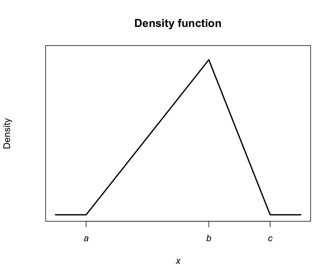
FIGURE 7.16: A triangular distribution.