11 Expectations for multivariate distributions*

11.1 Expectation

Results involving expectations naturally generalise from the bivariate to the multivariate case. Firstly, the expectation of a linear combination of random variables.

Theorem 11.1 (Expectation of linear combinations) If \(X_1, X_2,\dots, X_n\) are random variables and \(a_1, a_2,\ldots a_n\) are any constants then \[ \operatorname{E}\left[\sum_{i = 1}^n a_i X_i \right] =\sum_{i = 1}^n a_i \, \operatorname{E}[X_i] \]

Proof. The proof follows directly from Theorem 5.8 by induction.

The variance of a linear combination of random variables is given in the following theorem.

Theorem 11.2 (Variance of a linear combination) If \(X_1, X_2, \dots, X_n\) are random variables and \(a_1, a_2,\ldots a_n\) are any constants then \[ \operatorname{var}\left[\sum_{i = 1}^n a_i X_i \right] = \sum^n_{i = 1}a^2_i\operatorname{var}[X_i] + 2{\sum\sum}_{i<j}a_i a_j\operatorname{Cov}(X_i, X_j). \]

Proof. For convenience, put \(Y = \sum_{i = 1}^n a_iX_i\). Then by definition of variance \[\begin{align*} \operatorname{var}[Y] &= \operatorname{E}\big[Y - \operatorname{E}(Y)\big]^2\\ &= \operatorname{E}[a_1 X_1 + \dots + a_n X_n - a_1\mu_1 - \dots a_n\mu_n]^2\\ &= \operatorname{E}[a_1(X_1 - \mu_1) + \dots + a_n(X_n - \mu_n)]^2\\ &= \operatorname{E}\left[ \sum_i a^2_i(X_i - \mu_i)^2 + 2\mathop{\sum\sum}_{i < j}a_i a_j(X_i - \mu_i)X_j - \mu_j)\right]\\ &= \sum_i a^2_i\operatorname{E}[X_i - \mu_i]^2 + 2\mathop{\sum\sum}_{i < j}a_i a_j\operatorname{E}[X_i - \mu_i] (X_j - \mu_j)\\ %\quad \text{using Theorem\ \@ref(thm:ExpLinear)}\\ &= \sum_i a^2_i\sigma^2_i + 2\mathop{\sum\sum}_{i<j}a_i a_j\operatorname{Cov}(X_i, X_j). \end{align*}\]

In statistical theory, an important special case of Theorem 11.2 occurs when the \(X_i\) are independently and identically distributed (IID). That is, each of \(X_1, X_2, \dots, X_n\) has the same distribution and are independent of each other. (We see the relevance of this in Chap. 12.) Because of its importance this special case is called a corollary of Theorems 11.1 and 11.2.

Corollary 11.1 (IID rvs) If \(X_1, X_2, \dots, X_n\) are independently distributed (IID) random variables, each with mean \(\mu\) and variance \(\sigma^2\), and \(a_1, a_2,\ldots a_n\) are any constants, then \[\begin{align*} \operatorname{E}\left[\sum_{i = 1}^n a_i X_i \right] &= \mu\sum_{i = 1}^n a_i;\\ \operatorname{var}\left[\sum_{i = 1}^n a_i X_i \right] &= \sigma^2\sum^n_{i = 1}a^2_i. \end{align*}\]

Proof. Exercise!

11.2 Vector formulation

With the standard rules of matrix multiplication, Theorems 11.1 and 11.2 applied to Eq. (11.1) then give respectively (check!) \[\begin{equation} \operatorname{E}[Y] = \operatorname{E}[\mathbf{a}^T\mathbf{X}] = [a_1, a_2] \begin{bmatrix} \mu_1 \\ \mu_2 \end{bmatrix} = \mathbf{a}^T\boldsymbol{\mu} \end{equation}\] and \[\begin{align} \operatorname{var}[Y] &= \operatorname{var}[\mathbf{a}^T\mathbf{X}\mathbf{a}]\nonumber\\ &= [a_1, a_2] \begin{bmatrix} \sigma^2_1 & \sigma_{12} \\ \sigma_{21}& \sigma^2_2 \end{bmatrix} \begin{bmatrix} a_1 \\ a_2 \end{bmatrix} \nonumber\\ &= \mathbf{a}^T\mathbf{\Sigma}\mathbf{a}. \end{align}\]

The vector formulation of these results apply directly in the multivariate case as described below. Write \[\begin{align*} \mathbf{X} &= [X_1, X_2, \ldots, X_n]^T; \\ \operatorname{E}[\mathbf{X}] &= [\mu_1, \ldots, \mu_n]^T = \boldsymbol{\mu}^T; \\ \operatorname{var}[\mathbf{X}] &= \mathbf{\Sigma}; \\ \mathbf{a}^T & = \left[a_1,a_2,\ldots, a_n \right]. \end{align*}\] Now Theorems 11.1 and 11.2 can be expressed in vector form.

Theorem 11.3 (Bivariate mean and variance (vector form)) If \(\mathbf{X}\) is a random vector of length \(n\) with mean \(\boldsymbol{\mu}\) and variance \(\mathbf{\Sigma}\), and \(\mathbf{a}\) is any constant vector of length \(n\), then \[\begin{align*} \operatorname{E}[\mathbf{a}^T\mathbf{X}] &= \mathbf{a}^T\boldsymbol{\mu}; \\ \operatorname{var}[\mathbf{a}^T\mathbf{X}] &= \mathbf{a}^T\mathbf{\Sigma}\mathbf{a}. \end{align*}\]

Proof. Exercise.

These elegant statements concerning linear combinations are a feature of vector formulations that extend to many statistical results in the theory of statistics. One obvious advantage of this formulation is the implementation in vector-based computer programming used by packages such as R.

One further result is presented (without proof) involving two linear combinations.

Theorem 11.4 (Covariance of combinations) If \(\mathbf{X}\) is a random vector of length \(n\) with mean \(\boldsymbol{\mu}\) and variance \(\mathbf{\Sigma}\), and \(\mathbf{a}\) and \(\mathbf{b}\) are any constant vectors, each of length \(n\), then \[ \operatorname{Cov}(\mathbf{a}^T\mathbf{X},\mathbf{b}^T\mathbf{X}) = \mathbf{a}^T\mathbf{\Sigma}\mathbf{b}. \]

Example 11.1 (Expectations using vectors) Suppose the random variables \(X_1, X_2, X_3\) have respective means \(1\), \(2\), and \(3\), respective variances \(4\), \(5\), and \(6\), and covariances \(\operatorname{Cov}(X_1, X_2) = -1\), \(\operatorname{Cov}(X_1, X_3) = 1\) and \(\operatorname{Cov}(X_2, X_3) = 0\).

Consider the random variables \(Y_1 = 3X_1 + 2X_2 - X_3\) and \(Y_2 = X_3 - X_1\). Determine \(\operatorname{E}[Y_1]\), \(\operatorname{E}[Y_2]\), \(\operatorname{var}[Y_1]\), \(\operatorname{var}[Y_2]\) and \(\operatorname{Cov}(Y_1,Y_2)\).

A vector formulation of this problem allows us to use Theorems 11.3 and 11.4 directly. Putting \(\mathbf{a}^T = [3, 2, -1]\) and \(\mathbf{b}^T = [-1, 0, 1]\): \[ Y_1 = \mathbf{a}^T\mathbf{X} \quad\text{and}\quad Y_2 = \mathbf{b}^T\mathbf{X} \] where \(\mathbf{X}^T = [X_1, X_2, X_3]\). Also define \(\boldsymbol{\mu}^T = [1, 2, 3]\) and \(\mathbf{\Sigma} = \begin{bmatrix} 4 & -1 & 1\\ -1 & 5 & 0\\ 1 & 0 & 6 \end{bmatrix}\) as the mean and variance–covariance matrix respectively of \(\mathbf{X}\). Then \[ \operatorname{E}[Y_1] = \mathbf{a}^T\boldsymbol{\mu} = [3, 2, -1] \begin{bmatrix} 1\\ 2\\ 3 \end{bmatrix} = 4 \] and \[ \operatorname{var}[Y_1] = \mathbf{a}^T\mathbf{\Sigma}\mathbf{a} = [3, 2, -1] \begin{bmatrix} 4 & -1 & 1\\ -1 & 5 & 0\\ 1 & 0 & 6 \end{bmatrix} \begin{bmatrix} 3\\ 2\\ -1 \end{bmatrix} = 44. \] Similarly \(\operatorname{E}[Y_2] = 2\) and \(\operatorname{var}[Y_2] = 8\). Finally: \[ \operatorname{Cov}(Y_1, Y_2) = \mathbf{a}^T\mathbf{\Sigma}\mathbf{b} = [3, 2, -1]^T \begin{bmatrix} 4 & -1 & 1\\ -1 & 5 & 0\\ 1 & 0 & 6 \end{bmatrix} \begin{bmatrix} -1\\ 0\\ 1 \end{bmatrix} = -12. \]

11.3 Expectation and covariance

Consider a random vector of \(n\) random variables \[ \mathbf{X} = [X_1, X_2, \dots, X_n]^T. \] The mean vector of \(\mathbf{X}\) is \[ \boldsymbol{\mu} = E[\mathbf{X}] = \begin{bmatrix} E[X_1] \\ \vdots \\ E[X_n] \end{bmatrix}. \]

The covariance matrix is \[ \Sigma = \text{Cov}(\mathbf{X}) = E\!\left[(\mathbf{X} - \boldsymbol{\mu})(\mathbf{X} - \boldsymbol{\mu})^T\right]. \]

The entries are \(\Sigma_{ij} = \text{Cov}(X_i, X_j)\). The diagonal entries are variances, while the off-diagonal entries are covariances.

The correlation matrix is obtained by normalisation: \[ \rho_{ij} = \frac{\Sigma_{ij}}{\sqrt{\Sigma_{ii}\,\Sigma_{jj}}}. \]

11.4 Independence

The components \(X_1, \dots, X_n\) are independent if and only if \[ f(x_1, \dots, x_n) = \prod_{i = 1}^n f_{X_i}(x_i). \]

Linear combinations of random variables are most elegantly dealt with using the methods and notation of vectors and matrices, especially as the dimension grows beyond the bivariate case. In the bivariate case we define \[\begin{align} \mathbf{X} &= \begin{bmatrix} X_1 \\ X_2 \end{bmatrix}; \label{EQN:matrix1} \\ \operatorname{E}[\mathbf{X}] & = \operatorname{E} \left[ \begin{bmatrix} X_1 \\ X_2 \end{bmatrix} \right] = \begin{bmatrix} \operatorname{E}[X_1] \\ \operatorname{E}[X_2] \end{bmatrix} = \begin{bmatrix} \mu_1 \\ \mu_2 \end{bmatrix} = \boldsymbol{\mu};\label{EQN:matrix2} \\ \operatorname{var}[\mathbf{X}] & = \operatorname{var} \left[ \begin{bmatrix} X_1 \\ X_2 \end{bmatrix} \right] = \begin{bmatrix} \sigma^2_1 & \sigma_{12} \\ \sigma_{21} & \sigma^2_2 \end{bmatrix} = \mathbf{\Sigma}.\label{EQN:matrix3} \end{align}\]

The vector \(\boldsymbol{\mu}\) is the mean vector, and the matrix \(\mathbf{\Sigma}\) is called the variance–covariance matrix, which is square and symmetric since \(\sigma_{12} = \sigma_{21}\) (the covariance).

The linear combination \(Y = a_1 X_1 + a_2 X_2\) can be expressed as \[\begin{equation} Y = a_1 X_1 + a_2 X_2 = [a_1, a_2] \begin{bmatrix} X_1 \\ X_2 \end{bmatrix} = \mathbf{a}^T\mathbf{X} \tag{11.1} \end{equation}\] where the (column) vector \(\mathbf{a} = \begin{bmatrix} a_1 \\ a_2 \end{bmatrix}\), and the superscript \(T\) means ‘transpose’.

11.5 Independent random variables

Recall that events \(A\) and \(B\) are independent if, and only if, \[ something nmissing! \]

11.6 Simulation

As with univariate distributions (Sects. 7.11 and 8.10), simulation can be used with bivariate distributions. Random numbers from the bivariate normal distribution (Sect. 8.8) are generated using the function dmnorm() from the library mnorm. Random numbers from the multinomial distribution (Sect. 7.9) are generated using the function rmultinom(). More commonly, univariate distributions are combined.

Monthly rainfall, for example, is commonly modelled using gamma distributions (for example, Husak, Michaelsen, and Funk (2007)). Simulating rainfall is then used in others models (such as for cropping simulations; for example Ines and Hansen (2006)). As an example, consider a location where the monthly rainfall is well-modelled by a gamma distribution with a shape parameter \(\alpha = 1.6\) and a scale parameter of \(\beta = 220\) (Fig. 11.1, left panel):

library("mnorm") # Need to explicitly load  mnorm  library
MRain <- rgamma( 2000,
                 shape = 1.6,
                 scale = 220)

cat("Rainfall exceeding 900mm:",
    sum(MRain > 900) / 2000 * 100, "%\n")
#> Rainfall exceeding 900mm: 4.95 %
# Directly:
round( (1 - pgamma(900, shape = 1.6, scale = 220) ) * 100, 2)
#> [1] 4.95

The percentage of months with rainfall exceeding \(1000\,\text{mm}\) was also computed. However, now suppose that the shape parameter \(\alpha\) also varies, with an exponential distribution with mean \(2\) (Fig. 11.1, centre panel):

MRain2 <- rgamma( 1000,
                  shape = rexp(1000, rate = 1/2),
                  scale = 220)

cat("Rainfall exceeding 900mm:",
    sum(MRain2 > 900) / 1000 * 100, "%\n")
#> Rainfall exceeding 900mm: 13.3 %

Using simulation, it is also easy to simulate the impact of the scale parameter \(\beta\) varying also, suppose with a normal distribution mean of \(200\) and variance of \(16\) (Fig. 11.1, right panel):

MRain3 <- rgamma( 1000,
                  shape = rexp(1000, rate = 1/2),
                  scale = rnorm(1000, mean = 200, sd = 4))

cat("Rainfall exceeding 900:",
    sum(MRain3 > 900) / 1000 * 100, "%\n")
#> Rainfall exceeding 900: 11.4 %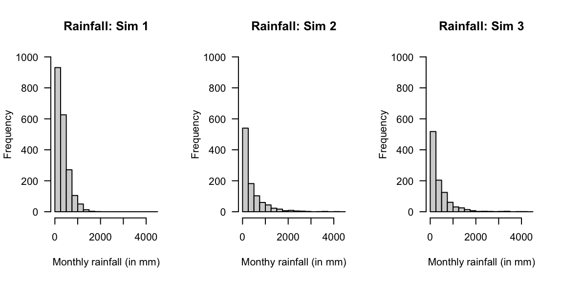

FIGURE 11.1: Three simulations using the gamma distribution.

11.7 Exercises

Selected answers appear in Sect. E.11.

Exercise 11.1 Suppose \(X_1, X_2, \dots, X_n\) are independently distributed random variables, each with mean \(\mu\) and variance \(\sigma^2\). Define the sample mean as \(\overline{X} = \left( \sum_{i=1}^n X_i\right)/n\).

1. Prove that \(\operatorname{E}[\overline{X}] = \mu\).
2. Find the variance of \(\overline{X}\).

Exercise 11.2 NO LONGER NEEDED:

The Poisson-gamma distributions (e.g., see Hasan and Dunn (2010b)), used for modelling rainfall, can be developed as follows:

• Let \(N\) be the number of rainfall events in a month, where \(N\sim \text{Pois}(\lambda)\). If no rainfall events are recorded in any month, then the monthly rainfall is \(Z = 0\).
• For each rainfall event (that is, when \(N > 0\)), say \(i\) for \(i = 1, 2, \dots N\), the amount of rain in event \(i\), say \(Y_i\), is modelled using a gamma distribution with parameter \(\alpha\) and \(\beta\).
• The total monthly rainfall is then \(Z = \sum_{i = 1}^N Y_i\).

Suppose the monthly rainfall station at a particular station can be modelled using \(\lambda = 0.78\), \(\alpha = 0.5\) and \(\beta = 6\).

1. Use a simulation to produce a one-month rainfall total using this model.
2. Repeat for \(1\,000\) simulations (i.e., simulate \(1\,000\) months), and plot the distribution.
3. What type of random variable is the monthly rainfall: discrete, continuous, or mixed? Explain.
4. Based on the \(1\,000\) simulations, approximately how often does a month have exactly zero rainfall?
5. Based on the \(1\,000\) simulations, what is the mean monthly rainfall?
6. Based on the \(1\,000\) simulations, what is the mean monthly rainfall in months where rain is recorded?

Exercise 11.3 \(X\), \(Y\) and \(Z\) are uncorrelated random variables with expected values \(\mu_x\), \(\mu_y\) and \(\mu_z\) and standard deviations \(\sigma_x\), \(\sigma_y\) and \(\sigma_z\). \(U\) and \(V\) are defined by \[\begin{align*} U&= X - Z;\\ V&= X - 2Y + Z. \end{align*}\]

1. Find the expected values of \(U\) and \(V\).
2. Find the variance of \(U\) and \(V\).
3. Find the covariance between \(U\) and \(V\).
4. Under what conditions on \(\sigma_x\), \(\sigma_y\) and \(\sigma_z\) are \(U\) and \(V\) uncorrelated?

Exercise 11.4 Suppose \((X, Y)\) has joint probability function given by \[ \Pr(X = x, Y = y) = \frac{|x - y|}{11} \] for \(x = 0, 1, 2\) and \(y = 1, 2, 3\).

1. Find \(\operatorname{E}[X \mid Y = 2]\).
2. Find \(\operatorname{E}[Y \mid X\ge 1]\).

Exercise 11.5 The PDF of \((X, Y)\) is given by \[ f_{X, Y}(x, y) = 1 - \alpha(1 - 2x)(1 - 2y), \] for \(0 \le x \le 1\), \(0 \le y \le 1\) and \(-1 \le \alpha \le 1\).

1. Find the marginal distributions of \(X\) and \(Y\).
2. Evaluate the correlation coefficient \(\rho_{XY}\).
3. For what value of \(\alpha\) are \(X\) and \(Y\) independent?
4. Find \(\Pr(X < Y)\).

Exercise 11.6 The random variables \(X_1\), \(X_2\), and \(X_3\) have y

• \(X_1\): mean \(\mu_1 = 5\) with standard deviation \(\sigma_1 = 2\).
• \(X_2\): mean \(\mu_2 = 3\) with standard deviation \(\sigma_2 = 3\).
• \(X_3\): mean \(\mu_3 = 6\) with standard deviation \(\sigma_3 = 4\).

The correlations are: \(\rho_{12} = -\frac{1}{6}\), \(\rho_{13} = \frac{1}{6}\) and \(\rho_{23} = \frac{1}{2}\).

If the random variables \(U\) and \(V\) are defined by \(U = 2X_1 + X_2 - X_3\) and \(V = X_1 - 2X_2 - X_3\), find

1. \(\operatorname{E}[U]\).
2. \(\operatorname{var}[U]\).
3. \(\operatorname{Cov}(U, V)\).

Exercise 11.7 Let \(X\) and \(Y\) be the body mass index (BMI) and percentage body fat for netball players attending the AIS. Assume \(X\) and \(Y\) have a bivariate normal distribution with \(\mu_X = 23\), \(\mu_Y = 21\), \(\sigma_X = 3\), \(\sigma_Y = 6\) and \(\rho_{XY} = 0.8\). Find

1. the expected BMI of a netball player who has a percent body fat of \(30\).
2. the expected percentage body fat of a netball player who has a BMI of \(19\).

Exercise 11.8 Let \(X\) and \(Y\) have a bivariate normal distribution with parameters \(\mu_x = 1\), \(\mu_y = 4\), \(\sigma^2_x = 4\), \(\sigma^2_y = 9\) and \(\rho = 0.6\). Find

1. \(\Pr(-1.5 < X < 2.5)\).
2. \(\Pr(-1.5 < X < 2.5 \mid Y = 3)\).
3. \(\Pr(0 < Y < 8)\).
4. \(\Pr(0 < Y < 8 \mid X = 0)\).

Exercise 11.9 Consider \(n\) random variables \(Z_i\) such that \(Z_i \sim \text{Exp}(\beta)\) for every \(i = 1, \dots, n\). Show that the distribution of \(Z_1 + Z_2 + \cdots + Z_n\) has a gamma distribution \(\text{Gam}(n, \beta)\), and determine the parameters of this gamma distribution. (Hint: See Theorem 5.6.)

Exercise 11.10 Daniel S. Wilks (1995b) (p. 101) states that the maximum daily temperatures measured at Ithaca (\(I\)) and Canandaigua (\(C\)) in January 1987 are both symmetrical. He also says that the two temperatures could be modelled with a bivariate normal distribution with \(\mu_I = 29.87\), \(\mu_C = 31.77\), \(\sigma_I = 7.71\), \(\sigma_C = 7.86\) and \(\rho_{IC} = 0.957\). (All measurements are in degrees Fahrenheit.)

1. Explain, in context, what a correlation coefficient of \(0.957\) means.
2. Determine the marginal distributions of \(C\) and of \(I\).
3. Find the conditional distribution of \(C\mid I\).
4. Plot the PDF of Canandaigua maximum temperature.
5. Plot the conditional PDF of Canandaigua maximum temperature given that the maximum temperature at Ithaca is \(25^\circ\)F.
6. Comment on the differences between the two PDFs plotted above.
7. Find \(\Pr(C < 32 \mid I = 25)\).
8. Find \(\Pr(C < 32)\).
9. Comment on the differences between the last two answers.
10. If temperature were measured in degrees Celsius instead of degrees Fahrenheit, how would the value of \(\rho_{IC}\) change?

Exercise 11.11 The discrete random variables \(X\) and \(Y\) have the joint probability distribution shown in the following table:

Value of \(x\)	\(y = 1\)	\(y = 2\)	\(y = 3\)
\(x = 0\)	0.20	0.15	0.05
\(x = 1\)	0.20	0.25	0.00
\(x = 3\)	0.10	0.05	0.00

1. Determine the marginal distribution of \(X\).
2. Calculate \(\Pr(X \ne Y)\).
3. Calculate \(\Pr(X + Y = 2 \mid X = Y)\).
4. Are \(X\) and \(Y\) independent? Justify your answer.
5. Calculate the correlation of \(X\) and \(Y\); i.e., compute \(\text{Cor}(X,Y)\).

Exercise 11.12 Suppose \(X\) and \(Y\) have the joint PDF \[ f_{X, Y}(x, y) = \frac{2 + x + y}{8} \quad\text{for $-1 < x < 1$ and $-1 < y < 1$}. \]

1. Sketch the distribution using R.
2. Determine the marginal PDF of \(X\).
3. Are \(X\) and \(Y\) independent? Give reasons.
4. Determine \(\Pr(X > 0, Y > 0)\).
5. Determine \(\Pr(X \ge 0, Y \ge 0, X + Y \le 1)\).
6. Determine \(\operatorname{E}[XY]\).
7. Determine \(\operatorname{var}[Y]\).
8. Determine \(\operatorname{Cov}(X, Y)\).

Exercise 11.13 Historically, final marks in a certain course are approximately normally distributed with mean of \(64\) and standard deviation \(8\). Out of fifteen students completing the course, what is the probability that \(2\) obtain HDs, \(3\) Distinctions, \(4\) Credits, \(5\) Passes and \(2\) Fails?

Exercise 11.14 Let \(X_1, X_2, X_3, \dots, X_n\) denote are independently and identically distributed with PDF \[ f_X(x) = 4x^3\quad \text{for $0 < x < 1$}. \]

1. Write down an expression for the joint PDF of distribution of \(X_1, X_2, X_3, \dots, X_n\).
2. Determine the probability that the first observation \(X_1\) is less than \(0.5\).
3. Determine the probability that all observations are less than \(0.5\).
4. Use the result above to deduce then the probability that the largest observation is less than \(0.5\).

Exercise 11.15 Let \(X\) and \(Y\) have a bivariate normal distribution with \(\operatorname{E}[X] = 5\), \(\operatorname{E}[Y] = -2\), \(\operatorname{var}[X] = 4\), \(\operatorname{var}[Y] = 9\), and \(\operatorname{Cov}(X, Y) = -3\). Determine the joint distribution of \(U = 3X + 4Y\) and \(V = 5X - 6Y\).

Exercise 11.16 Two fair dice are rolled. Let \(X\) and \(Y\) denote, respectively, the maximum and minimum of the numbers of spots showing on the two dice.

1. Construct a table that enumerates the sample space.
2. Determine \(E(Y\mid X = 4)\) for \(1\le x\le 6\).
3. Simulate this experiment using R. Compare the simulated results with the theoretical results found above.

Exercise 11.17 Let \(X\) be a random variable for which \(\operatorname{E}[X] = \mu\) and \(\operatorname{var}[X] = \sigma^2\), and let \(c\) be an arbitrary constant.

1. Show that \[ \operatorname{E}[(X - c)^2] = (\mu - c)^2 + \sigma^2. \]
2. What does the result above tell us about the possible size of \(\operatorname{E}[(X - c)^2]\)?

Exercise 11.18 In Sect. 11.6, simulation was used for monthly rainfall. Daily rainfall, however, is more difficult to model as some days have exactly zero rainfall, and on some days a continuous amount of rainfalls; i.e., daily monthly is a mixed random variable (Sect. 3.2.3).

One way to model daily rainfall is to use a two-step process (Chandler and Wheater 2002). Firstly, model whether a day records rainfall or not (using a binomial distribution): the occurrence model. Then, for days on which rain falls, model the amount of rainfall using a gamma distribution: the amounts model.

1. Use this information to model daily rainfall over one year (\(365\) days), for a location where the probability of a wet day is \(0.32\), and the amount of rainfall on wet days follows a gamma distribution with \(\alpha = 2\) and \(\beta = 20\). Produce a histogram of the distribution of annual rainfall after \(1\,000\) simulations.
2. Suppose that the probability of rainfall, \(p\), depends on the day of the year, such that: \[ p = \left\{1 + \cos[ 2\pi\times(\text{day of year})/365]\right\} / 2.2. \] Plot the change in \(p\) over the day of the year.
3. Revise the first model using this value of \(p\). Produce a histogram of the distribution of annual rainfall after \(1\,000\) simulations.
4. Revise the initial model (where the probability of rain of Day 1 is still \(0.32\)), so that the value of \(p\) depends on what happened the day before: If day \(i\) receives rain, then the probability that the following day receives rain is \(p = 0.55\); if day \(i\) does not receive rain, then the probability that the following day receives rain is just \(p = 0.15\). Produce a histogram of the distribution of annual rainfall after \(1\,000\) simulations.

Exercise 11.19 A company produces a \(500\,\text{g}\) packet of ‘trail mix’ that includes a certain weight of nuts \(X\), dried fruit \(Y\), and seeds \(Z\). The actually weights of each ingredient vary randomly, depending on seasonality and availability.

1. Explain why there are really just two variables in this problem.
2. Suppose the weight of nuts plus dried fruit must be between \(300\,\text{g}\) and \(400\,\text{g}\). Draw the sample space.
3. In addition, suppose the weight of nuts must be at least \(100\,\text{g}\), and the weight of dried fruit must be at least \(100\,\text{g}\). Draw the sample space.
4. Under the above conditions, assume the weights of ingredients used in the trail mix are uniformly distributed. Determine the probability function.

Exercise 11.20 Mixed nuts come in \(250\,\text{g}\) packets, and comprise walnuts, almonds and peanuts. The actual weights of each ingredient vary randomly, depending on seasonality and availability.

1. Explain why there are really just two variables in this problem.
2. While peanuts are the cheapest ingredient, guidelines state that the weight of peanuts must not exceed \(100\,\text{g}\). Draw the sample space.
3. In addition, suppose the weight of almonds must be at least \(25\,\text{g}\), and the weight of walnuts must be at least \(25\,\text{g}\). Draw the sample space.
4. Under the above conditions, assume the weights of ingredients used in the mixed nuts packets are uniformly distributed. Determine the probability function.

Exercise 11.21 Suppose \(X\) is the concentration of a biomarker (in mmol.L^\(-1\)), and \(Y\) is a disease indicator where \(Y = 1\) refers to a patient with the disease and \(Y = 0\) refers to a patient without the disease.
The prevalence of the disease in the population is \[ \Pr(Y = 1) = 0.10, \quad \Pr(Y = 0) = 0.90. \] Conditional on disease status, biomarker concentrations follow different ??????normal?????? distributions. If \(Y = 1\):
\[ X \mid Y = 1 \sim \mathcal{N}(\mu_1=8, \, \sigma_1^2 = 1^2), \] and if \(Y = 0\): \[ X \mid Y = 0 \sim \mathcal{N}(\mu_0=5, \, \sigma_0^2 = 1^2). \] 1. Write down the joint density–mass function \(f_{X, Y}(x, y)\).
2. Derive the marginal density of \(X\), \(f_X(x)\).
3. Compute \(\Pr(Y = 1 \mid X = 7)\) (the posterior probability of disease given biomarker level \(7\)).
4. Interpret this probability in plain language.

Exercise 11.22 A machine component can fail for one of three reasons:

• mechanical failure (\(Y = 1\)), with probability \(0.5\);
• electrical failure (\(Y = 2\)), with probability \(0.3\);
• thermal failure (\(Y = 3\)), with probability \(0.2\).

The random variable \(X\) denotes the time to failure (in hundreds of hours). Conditional on knowing the mode of failure, the time-to-failure has the distribution \[ f_{X\mid Y}(x\mid Y = y) = \lambda_y \exp(-\lambda_y x) \quad\text{for $x > 0$} \] where

• \(\lambda_y = 1\) if the failure is mechanical;
• \(\lambda_y = 0.5\) if the failure is electrical; and
• \(\lambda_y = 0.25\) if the failure is thermal.

1. Write down the joint density–mass function \(f_{X, Y}(x, y)\).
2. Find the marginal density of the time to failure \(f_X(x)\).
3. Compute \(\Pr(Y = 1 \mid X \leq 2)\), the probability that the failure mode was mechanical given that the component failed within \(200\) hours.
4. Interpret the result in words.

---

Peter K. Dunn, 2024: CC BY-NC-SA 4.0